PDF version (NAG web site
, 64-bit version, 64-bit version)
NAG Toolbox: nag_ode_ivp_rk_zero_simple (d02bj)
Purpose
nag_ode_ivp_rk_zero_simple (d02bj) integrates a system of first-order ordinary differential equations over an interval with suitable initial conditions, using a fixed order Runge–Kutta method, until a user-specified function, if supplied, of the solution is zero, and returns the solution at points specified by you, if desired.
Syntax
[
x,
y,
ifail] = d02bj(
x,
xend,
y,
fcn,
tol,
relabs,
output,
g, 'n',
n)
[
x,
y,
ifail] = nag_ode_ivp_rk_zero_simple(
x,
xend,
y,
fcn,
tol,
relabs,
output,
g, 'n',
n)
Description
nag_ode_ivp_rk_zero_simple (d02bj) advances the solution of a system of ordinary differential equations
from
to
using a fixed order Runge–Kutta method. The system is defined by
fcn, which evaluates
in terms of
and
. The initial values of
must be given at
.
The solution is returned via the
output supplied by you and at points specified by you, if desired: this solution is obtained by
interpolation on solution values produced by the method. As the integration proceeds a check can be made on the user-specified function
to determine an interval where it changes sign. The position of this sign change is then determined accurately by
interpolation to the solution. It is assumed that
is a continuous function of the variables, so that a solution of
can be determined by searching for a change in sign in
. The accuracy of the integration, the interpolation and, indirectly, of the determination of the position where
, is controlled by the arguments
tol and
relabs.
References
Shampine L F (1994) Numerical solution of ordinary differential equations Chapman and Hall
Parameters
Compulsory Input Parameters
- 1:
– double scalar
-
The initial value of the independent variable .
- 2:
– double scalar
-
The final value of the independent variable. If , integration will proceed in the negative direction.
Constraint:
.
- 3:
– double array
-
The initial values of the solution at .
- 4:
– function handle or string containing name of m-file
-
fcn must evaluate the functions
(i.e., the derivatives
) for given values of its arguments
.
[f] = fcn(x, y)
Input Parameters
- 1:
– double scalar
-
, the value of the independent variable.
- 2:
– double array
-
, for , the value of the variable.
Output Parameters
- 1:
– double array
-
The value of
, for .
- 5:
– double scalar
-
A
positive tolerance for controlling the error in the integration. Hence
tol affects the determination of the position where
, if
is supplied.
nag_ode_ivp_rk_zero_simple (d02bj) has been designed so that, for most problems, a reduction in
tol leads to an approximately proportional reduction in the error in the solution. However, the actual relation between
tol and the accuracy achieved cannot be guaranteed. You are strongly recommended to call
nag_ode_ivp_rk_zero_simple (d02bj) with more than one value for
tol and to compare the results obtained to estimate their accuracy. In the absence of any prior knowledge, you might compare the results obtained by calling
nag_ode_ivp_rk_zero_simple (d02bj) with
and with each of
and
where
correct significant digits are required in the solution,
. The accuracy of the value
such that
is indirectly controlled by varying
tol. You should experiment to determine this accuracy.
Constraint:
.
- 6:
– string (length ≥ 1)
-
The type of error control. At each step in the numerical solution an estimate of the local error,
, is made. For the current step to be accepted the following condition must be satisfied:
where
and
are defined by
where
and
are small machine-dependent numbers and
is an estimate of the local error at
, computed internally. If the condition is not satisfied, the step size is reduced and the solution is recomputed on the current step. If you wish to measure the error in the computed solution in terms of the number of correct decimal places, then
relabs should be set to 'A' on entry, whereas if the error requirement is in terms of the number of correct significant digits, then
relabs should be set to 'R'. If you prefer a mixed error test, then
relabs should be set to 'M', otherwise if you have no preference,
relabs should be set to the default 'D'. Note that in this case 'D' is taken to be 'R'.
Constraint:
, , or .
- 7:
– function handle or string containing name of m-file
-
output permits access to intermediate values of the computed solution (for example to print or plot them), at successive user-specified points. It is initially called by
nag_ode_ivp_rk_zero_simple (d02bj) with
(the initial value of
). You must reset
xsol to the next point (between the current
xsol and
xend) where
output is to be called, and so on at each call to
output. If, after a call to
output, the reset point
xsol is beyond
xend,
nag_ode_ivp_rk_zero_simple (d02bj) will integrate to
xend with no further calls to
output; if a call to
output is required at the point
, then
xsol must be given precisely the value
xend.
[xsol] = output(xsol, y)
Input Parameters
- 1:
– double scalar
-
The output value of the independent variable .
- 2:
– double array
-
The computed solution at the point
xsol.
Output Parameters
- 1:
– double scalar
-
You must set
xsol to the next value of
at which
output is to be called.
If you do not wish to access intermediate output, the actual argument
output
must be the string
nag_ode_ivp_rk_zero_simple_dummy_output (d02bjx). (
nag_ode_ivp_rk_zero_simple_dummy_output (d02bjx) is included in the NAG Toolbox.)
- 8:
– function handle or string containing name of m-file
-
g must evaluate the function
for specified values
. It specifies the function
for which the first position
where
is to be found.
[result] = g(x, y)
Input Parameters
- 1:
– double scalar
-
, the value of the independent variable.
- 2:
– double array
-
, for , the value of the variable.
Output Parameters
- 1:
– double scalar
-
The value of at the specified point.
If you do not require the root-finding option, the actual argument
g must be the string
nag_ode_ivp_rk_zero_simple_dummy_g (d02bjw). (
nag_ode_ivp_rk_zero_simple_dummy_g (d02bjw) is included in the NAG Toolbox.)
Optional Input Parameters
- 1:
– int64int32nag_int scalar
-
Default:
the dimension of the array
y.
, the number of equations.
Constraint:
.
Output Parameters
- 1:
– double scalar
-
If
is supplied by you, it contains the point where
, unless
anywhere on the range
x to
xend, in which case,
x will contain
xend (and the error indicator
is set); if
is not supplied by you it contains
xend. However, if an error has occurred, it contains the value of
at which the error occurred.
- 2:
– double array
-
The computed values of the solution at the final point .
- 3:
– int64int32nag_int scalar
unless the function detects an error (see
Error Indicators and Warnings).
Error Indicators and Warnings
Errors or warnings detected by the function:
-
-
| On entry, | , |
| or | tol is too small |
| or | , |
| or | , , or , |
| or | . |
-
-
With the given value of
tol, no further progress can be made across the integration range from the current point
. (See
Further Comments for a discussion of this error exit.) The components
contain the computed values of the solution at the current point
. If you have supplied
, then no point at which
changes sign has been located up to the point
.
-
-
tol is too small for
nag_ode_ivp_rk_zero_simple (d02bj) to take an initial step.
x and
retain their initial values.
-
-
xsol has not been reset or
xsol lies behind
x in the direction of integration, after the initial call to
output, if the
output option was selected.
-
-
A value of
xsol returned by the
output has not been reset or lies behind the last value of
xsol in the direction of integration, if the
output option was selected.
-
-
At no point in the range
x to
xend did the function
change sign, if
was supplied. It is assumed that
has no solution.
-
-
A serious error has occurred in an internal call to an interpolation function. Check all (sub)program calls and array dimensions. Seek expert help.
-
An unexpected error has been triggered by this routine. Please
contact
NAG.
-
Your licence key may have expired or may not have been installed correctly.
-
Dynamic memory allocation failed.
Accuracy
The accuracy of the computation of the solution vector
y may be controlled by varying the local error tolerance
tol. In general, a decrease in local error tolerance should lead to an increase in accuracy. You are advised to choose
unless you have a good reason for a different choice.
If the problem is a root-finding one, then the accuracy of the root determined will depend on the properties of
and on the values of
tol and
relabs. You should try to code
g without introducing any unnecessary cancellation errors.
Further Comments
If more than one root is required, then to determine the second and later roots
nag_ode_ivp_rk_zero_simple (d02bj) may be called again starting a short distance past the previously determined roots. Alternatively you may construct your own root-finding code using
nag_roots_contfn_brent_rcomm (c05az),
nag_ode_ivp_rkts_onestep (d02pf) and
nag_ode_ivp_rkts_interp (d02ps).
If
nag_ode_ivp_rk_zero_simple (d02bj) fails with
, then it can be called again with a larger value of
tol if this has not already been tried. If the accuracy requested is really needed and cannot be obtained with this function, the system may be very stiff (see below) or so badly scaled that it cannot be solved to the required accuracy.
If
nag_ode_ivp_rk_zero_simple (d02bj) fails with
, it is probable that it has been called with a value of
tol which is so small that a solution cannot be obtained on the range
x to
xend. This can happen for well-behaved systems and very small values of
tol. You should, however, consider whether there is a more fundamental difficulty. For example:
| (a) |
in the region of a singularity (infinite value) of the solution, the function will usually stop with , unless overflow occurs first. Numerical integration cannot be continued through a singularity, and analytic treatment should be considered; |
| (b) |
for ‘stiff’ equations where the solution contains rapidly decaying components, the function will use very small steps in (internally to nag_ode_ivp_rk_zero_simple (d02bj)) to preserve stability. This will exhibit itself by making the computing time excessively long, or occasionally by an exit with . Runge–Kutta methods are not efficient in such cases, and you should try nag_ode_ivp_bdf_zero_simple (d02ej). |
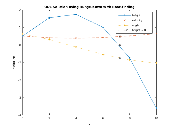
Example
This example illustrates the solution of four different problems. In each case the differential system (for a projectile) is
over an interval
to
starting with values
,
and
. We solve each of the following problems with local error tolerances
and
.
| (i) |
To integrate to producing intermediate output at intervals of until a root is encountered where . |
| (ii) |
As (i) but with no intermediate output. |
| (iii) |
As (i) but with no termination on a root-finding condition. |
| (iv) |
As (i) but with no intermediate output and no root-finding termination condition. |
Open in the MATLAB editor:
d02bj_example
function d02bj_example
fprintf('d02bj example results\n\n');
global ykeep ncall xkeep;
x = 0;
xend = 10;
y = [0.5; 0.5; pi/5];
relabs = 'Default';
xOut1 = [];
ncall = 0;
ykeep = zeros(1,length(y));
xkeep = zeros(1,1);
fprintf('Case 1: intermediate output, root-finding\n\n');
for j = 4:5
tol = double(10)^(-j);
disp(['Calculation with tol = ',num2str(tol)]);
disp(' X Y(1) Y(2) Y(3)');
[xOut, yOut, ifail] = d02bj(x, xend, y, @fcn, tol, ...
relabs, @output, @g);
disp(' ');
disp(['Root of Y(1) = 0.0 at ',num2str(xOut)]);
disp('Solution is' );
fprintf(' %8.4f %8.4f %8.4f\n\n', yOut);
end
fprintf('Case 2: no intermediate output, root-finding \n\n');
for j = 4:5
tol = double(10)^(-j);
disp(['Calculation with tol = ',num2str(tol)]);
[xOut, yOut, ifail] = d02bj(x, xend, y, @fcn, tol, ...
relabs, 'd02bjx',@g);
disp(['Root of Y(1) = 0.0 at ',num2str(xOut)]);
disp('Solution is' );
fprintf(' %8.4f %8.4f %8.4f\n\n', yOut);
xOut1 = xOut;
end
fprintf('Case 3: intermediate output, no root-finding\n\n');
for j = 4:5
tol = double(10)^(-j);
disp(['Calculation with tol = ',num2str(tol)]);
fprintf(' X Y(1) Y(2) Y(3) \n');
[xOut, yOut, ifail] = d02bj(x, xend, y, @fcn, tol, ...
relabs, @save,'d02bjw');
fprintf('\n');
end
fprintf(['Case 4: no intermediate output, no root-finding ', ...
'(integrate to xend)\n\n']);
for j = 4:5
tol = double(10)^(-j);
disp(['Calculation with tol = ',num2str(tol)]);
disp(' X Y(1) Y(2) Y(3)');
fprintf('%2d %8.4f %8.4f %8.4f\n', x, y);
[xOut, yOut, ifail] = ...
d02bj(x, xend, y, @fcn, tol, relabs, 'd02bjx','d02bjw');
fprintf('%2d %8.4f %8.4f %8.4f\n\n', xOut, yOut);
end
nres = 0.5*length(xkeep);
xplot = xkeep(nres+1:2*nres);
yplot = ykeep(nres+1:2*nres, :);
fig1 = figure;
display_plot(xplot, yplot, xOut1)
function xsolOut = save(xsol, y)
global ykeep ncall xkeep;
ncall = ncall+1;
ykeep(ncall,:) = y;
xkeep(ncall,:) = xsol;
fprintf('%2d %8.4f %8.4f %8.4f\n', xsol, y);
xsolOut = xsol + 2;
function xsolOut = output(xsol, y)
fprintf('%2d %8.4f %8.4f %8.4f\n', xsol, y);
xsolOut = xsol + 2;
function f = fcn(x,y)
f = zeros(3,1);
f(1) = tan(y(3));
f(2) = -0.032*tan(y(3))/y(2) - 0.02*y(2)/cos(y(3));
f(3) = -0.032/y(2)^2;
function result = g(x,y)
result = y(1);
function display_plot(xplot, yplot, xOut1)
plot(xplot, yplot(:,1), '-+', ...
xplot, yplot(:,2), '--x', ...
xplot, yplot(:,3), ':*');
do_stem(xplot, yplot, xOut1);
title('ODE Solution using Runge-Kutta with Root-finding');
xlabel('x');
ylabel('Solution');
legend('height','velocity','angle','height = 0','Location','Best');
function do_stem(xplot, yplot, xOut1)
for i = 1:length(xplot)
if xplot(i) > xOut1
break
end
end
dx = xplot(i)-xplot(i-1);
ddx = xOut1-xplot(i-1);
d1 = ddx/dx;
f1 = yplot(i-1,2) + d1*(yplot(i,2)-yplot(i-1,2));
f2 = yplot(i-1,3) + d1*(yplot(i,3)-yplot(i-1,3));
hold on
stem([xOut1,xOut1],[f1,0],'k:s');
hold on
stem([xOut1,xOut1],[f2,0],'k:s');
d02bj example results

Case 1: intermediate output, root-finding

Calculation with tol = 0.0001
 X     Y(1)       Y(2)       Y(3)
 0     0.5000     0.5000     0.6283
 2     1.5493     0.4055     0.3066
 4     1.7423     0.3743    -0.1289
 6     1.0055     0.4173    -0.5507

Root of Y(1) = 0.0 at 7.2882
Solution is
   -0.0000     0.4749    -0.7601

Calculation with tol = 1e-05
 X     Y(1)       Y(2)       Y(3)
 0     0.5000     0.5000     0.6283
 2     1.5493     0.4055     0.3066
 4     1.7423     0.3743    -0.1289
 6     1.0055     0.4173    -0.5507

Root of Y(1) = 0.0 at 7.2883
Solution is
   -0.0000     0.4749    -0.7601

Case 2: no intermediate output, root-finding

Calculation with tol = 0.0001
Root of Y(1) = 0.0 at 7.2882
Solution is
   -0.0000     0.4749    -0.7601

Calculation with tol = 1e-05
Root of Y(1) = 0.0 at 7.2883
Solution is
   -0.0000     0.4749    -0.7601

Case 3: intermediate output, no root-finding

Calculation with tol = 0.0001
 X     Y(1)       Y(2)       Y(3)
 0     0.5000     0.5000     0.6283
 2     1.5493     0.4055     0.3066
 4     1.7423     0.3743    -0.1289
 6     1.0055     0.4173    -0.5507
 8    -0.7460     0.5130    -0.8537
10    -3.6283     0.6333    -1.0515

Calculation with tol = 1e-05
 X     Y(1)       Y(2)       Y(3)
 0     0.5000     0.5000     0.6283
 2     1.5493     0.4055     0.3066
 4     1.7423     0.3743    -0.1289
 6     1.0055     0.4173    -0.5507
 8    -0.7459     0.5130    -0.8537
10    -3.6282     0.6333    -1.0515

Case 4: no intermediate output, no root-finding (integrate to xend)

Calculation with tol = 0.0001
 X     Y(1)       Y(2)       Y(3)
 0     0.5000     0.5000     0.6283
10    -3.6283     0.6333    -1.0515

Calculation with tol = 1e-05
 X     Y(1)       Y(2)       Y(3)
 0     0.5000     0.5000     0.6283
10    -3.6282     0.6333    -1.0515
PDF version (NAG web site
, 64-bit version, 64-bit version)
© The Numerical Algorithms Group Ltd, Oxford, UK. 2009–2015