PDF version (NAG web site
, 64-bit version, 64-bit version)
NAG Toolbox: nag_ode_bvp_shoot_genpar_algeq (d02sa)
Purpose
nag_ode_bvp_shoot_genpar_algeq (d02sa) solves a two-point boundary value problem for a system of first-order ordinary differential equations with boundary conditions, combined with additional algebraic equations. It uses initial value techniques and a modified Newton iteration in a shooting and matching method.
Syntax
[
p,
pf,
dp,
swp,
w,
ifail] = d02sa(
p,
n1,
pe,
pf,
e,
dp,
swp,
icount,
range,
bc,
fcn,
eqn,
constr,
ymax,
monit,
prsol, 'm',
m, 'n',
n, 'npoint',
npoint)
[
p,
pf,
dp,
swp,
w,
ifail] = nag_ode_bvp_shoot_genpar_algeq(
p,
n1,
pe,
pf,
e,
dp,
swp,
icount,
range,
bc,
fcn,
eqn,
constr,
ymax,
monit,
prsol, 'm',
m, 'n',
n, 'npoint',
npoint)
Note: the interface to this routine has changed since earlier releases of the toolbox:
| At Mark 22: |
npoint was made optional |
Description
nag_ode_bvp_shoot_genpar_algeq (d02sa) solves a two-point boundary value problem for a system of
first-order ordinary differential equations with separated boundary conditions by determining certain unknown arguments
. (There may also be additional algebraic equations to be solved in the determination of the arguments and, if so, these equations are defined by
eqn.) The arguments may be, but need not be, boundary values; they may include eigenvalues, arguments in the coefficients of the differential equations, coefficients in series expansions or asymptotic expansions for boundary values, the length of the range of definition of the system of differential equations, etc.
It is assumed that we have a system of
differential equations of the form
where
is the vector of arguments, and that the derivative
is evaluated by
fcn. Also,
of the equations are assumed to depend on
. For
the
equations of the system are not involved in the matching process. These are the driving equations; they should be independent of
and of the solution of the other
equations. In numbering the equations in
fcn and
bc the driving equations must be put
first (as they naturally occur in most applications). The range of definition [
] of the differential equations is defined by
range and may depend on the arguments
(that is, on
).
range must define the points
,
, which must satisfy
(or a similar relationship with all the inequalities reversed).
If
the points
can be used to break up the range of definition. Integration is restarted at each of these points. This means that the differential equations
(1) can be defined differently in each sub-interval
, for
. Also, since initial and maximum integration step sizes can be supplied on each sub-interval (via the array
swp), you can indicate parts of the range
where the solution
may be difficult to obtain accurately and can take appropriate action.
The boundary conditions may also depend on the arguments and are applied at
and
. They are defined (in
bc) in the form
The boundary value problem is solved by determining the unknown arguments
by a shooting and matching technique. The differential equations are always integrated from
to
with initial values
. The solution vector thus obtained at
is subtracted from the vector
to give the
residuals
, ignoring the first
, driving equations. Because the direction of integration is always from
to
, it is unnecessary, in
bc, to supply values for the first
boundary values at
, that is the first
components of
in
(3). For
then
. Together with the
equations defined by
eqn,
these give a vector of residuals
, which at the solution,
, must satisfy
These equations are solved by a pseudo-Newton iteration which uses a modified singular value decomposition of
when solving the linear equations which arise. The Jacobian
used in Newton's method is obtained by numerical differentiation. The arguments at each Newton iteration are accepted only if the norm
is much reduced from its previous value. Here
is the pseudo-inverse, calculated from the singular value decomposition, of a modified version of the Jacobian
(
is actually the inverse of the Jacobian in well-conditioned cases).
is a diagonal matrix with
where
pf is an array of floor values.
See
Deuflhard (1974) for further details of the variants of Newton's method used,
Gay (1976) for the modification of the singular value decomposition and
Gladwell (1979) for an overview of the method used.
Two facilities are provided to prevent the pseudo-Newton iteration running into difficulty. First, you are permitted to specify constraints on the values of the arguments
via a
constr. These constraints are only used to prevent the Newton iteration using values for
which would violate them; that is, they are not used to determine the values of
. Secondly, you are permitted to specify a maximum value
for
at all points in the range
. It is intended that this facility be used to prevent machine ‘overflow’ in the integrations of equation
(1) due to poor choices of the arguments
which might arise during the Newton iteration. When using this facility, it is presumed that you have an estimate of the likely size of
at all points
.
should then be chosen rather larger (say by a factor of
) than this estimate.
You are strongly advised to supply a
monit (or to call the ‘default’ function
nag_ode_bvp_shoot_genpar_algeq_sample_monit (d02hbx), see
monit) to monitor the progress of the pseudo-Newton iteration. You can output the solution of the problem
by supplying a suitable
prsol (an example is given in
Example of a function designed to output the solution at equally spaced points).
nag_ode_bvp_shoot_genpar_algeq (d02sa) is designed to try all possible options before admitting failure and returning to you. Provided the function can start the Newton iteration from the initial point it will exhaust all the options available to it (though you can override this by specifying a maximum number of iterations to be taken). The fact that all its options have been exhausted is the only error exit from the iteration. Other error exits are possible, however, whilst setting up the Newton iteration and when computing the final solution.
If you require more background information about the solution of boundary value problems by shooting methods you are recommended to read the appropriate chapters of
Hall and Watt (1976), and for a detailed description of
nag_ode_bvp_shoot_genpar_algeq (d02sa)
Gladwell (1979) is recommended.
References
Deuflhard P (1974) A modified Newton method for the solution of ill-conditioned systems of nonlinear equations with application to multiple shooting Numer. Math. 22 289–315
Gay D (1976) On modifying singular values to solve possibly singular systems of nonlinear equations Working Paper 125 Computer Research Centre, National Bureau for Economics and Management Science, Cambridge, MA
Gladwell I (1979) The development of the boundary value codes in the ordinary differential equations chapter of the NAG Library Codes for Boundary Value Problems in Ordinary Differential Equations. Lecture Notes in Computer Science (eds B Childs, M Scott, J W Daniel, E Denman and P Nelson) 76 Springer–Verlag
Hall G and Watt J M (ed.) (1976) Modern Numerical Methods for Ordinary Differential Equations Clarendon Press, Oxford
Parameters
Compulsory Input Parameters
- 1:
– double array
-
must be set to an estimate of the th argument, , for .
- 2:
– int64int32nag_int scalar
-
, the number of differential equations active in the matching process. The active equations must be placed last in the numbering in
fcn and
bc. The
first equations are used as the driving equations.
Constraint:
, and .
- 3:
– double array
-
, for
, must be set to a positive value for use in the convergence test in the
th argument
. See the description of
pf for further details.
Constraint:
, for .
- 4:
– double array
-
, for
, should be set to a ‘floor’ value in the convergence test on the
th argument
. If
on entry then it is set to the small positive value
(where
may in most cases be considered to be
machine precision); otherwise it is used unchanged.
The Newton iteration is presumed to have converged if a full Newton step is taken (
in the specification of
monit), the singular values of the Jacobian are not being significantly perturbed (also see
monit) and if the Newton correction
satisfies
where
is the current value of the
th argument. The values
are also used in determining the Newton iterates as discussed in
Description, see equation
(6).
- 5:
– double array
Default:
Values for use in controlling the local error in the integration of the differential equations. If
is an estimate of the local error in
, for
, then
where
may in most cases be considered to be
machine precision.
Constraint:
, for .
- 6:
– double array
-
A value to be used in perturbing the argument
in the numerical differentiation to estimate the Jacobian used in Newton's method. If
on entry, an estimate is made internally by setting
where
is the initial value of the argument supplied by you and
may in most cases be considered to be
machine precision. The estimate of the Jacobian,
, is made using forward differences, that is for each
, for
,
is perturbed to
and the
th column of
is estimated as
where the other components of
are unchanged (see
(3) for the notation used). If this fails to produce a Jacobian with significant columns, backward differences are tried by perturbing
to
and if this also fails then central differences are used with
perturbed to
. If this also fails then the calculation of the Jacobian is abandoned. If the Jacobian has not previously been calculated then an error exit is taken. If an earlier estimate of the Jacobian is available then the current argument set,
, for
, is abandoned in favour of the last argument set from which useful progress was made and the singular values of the Jacobian used at the point are modified before proceeding with the Newton iteration. You are recommended to use the default value
unless you have prior knowledge of a better choice. If any of the perturbations described are likely to lead to an unfortunate set of argument values then you should use
constr to prevent such perturbations (all changes of arguments are checked by a call to
constr).
- 7:
– double array
-
ldswp, the first dimension of the array, must satisfy the constraint
.
must contain an estimate for an initial step size for integration across the
th sub-interval
, for
, (see
range).
should have the same sign as
if it is nonzero. If
, on entry, a default value for the initial step size is calculated internally. This is the recommended mode of entry.
must contain a lower bound for the modulus of the step size on the
th sub-interval , for . If on entry, a very small default value is used. By setting but smaller than the expected step sizes (assuming you have some insight into the likely step sizes) expensive integrations with arguments far from the solution can be avoided.
must contain an upper bound on the modulus of the step size to be used in the integration on , for . If on entry no bound is assumed. This is the recommended mode of entry unless the solution is expected to have important features which might be ‘missed’ in the integration if the step size were permitted to be chosen freely.
- 8:
– int64int32nag_int scalar
-
An upper bound on the number of Newton iterations. If on entry, no check on the number of iterations is made (this is the recommended mode of entry).
Constraint:
.
- 9:
– function handle or string containing name of m-file
-
range must specify the break-points
, for
, which may depend on the arguments
, for
.
[x] = range(npoint, p, m)
Input Parameters
- 1:
– int64int32nag_int scalar
-
plus the number of break-points in .
- 2:
– double array
-
The current estimate of the
th argument, for .
- 3:
– int64int32nag_int scalar
-
, the number of arguments.
Output Parameters
- 1:
– double array
-
The
th break-point, for
. The sequence
must be strictly monotonic, that is either
or
- 10:
– function handle or string containing name of m-file
-
bc must place in
g1 and
g2 the boundary conditions at
and
respectively.
[g1, g2] = bc(p, m, n)
Input Parameters
- 1:
– double array
-
An estimate of the
th argument, , for .
- 2:
– int64int32nag_int scalar
-
, the number of arguments.
- 3:
– int64int32nag_int scalar
-
, the number of differential equations.
Output Parameters
- 1:
– double array
-
The value of
, for , (where this may be a known value or a function of the parameters
, for ).
- 2:
– double array
-
The value of
, for
, (where these may be known values or functions of the parameters
, for
). If
, so that there are some driving equations, then the first
values of
g2 need not be set since they are never used.
- 11:
– function handle or string containing name of m-file
-
fcn must evaluate the functions
(i.e., the derivatives
), for
.
[f] = fcn(x, y, n, p, m, ii)
Input Parameters
- 1:
– double scalar
-
, the value of the argument.
- 2:
– double array
-
, for , the value of the argument.
- 3:
– int64int32nag_int scalar
-
, the number of equations.
- 4:
– double array
-
The current estimate of the
th argument , for .
- 5:
– int64int32nag_int scalar
-
, the number of arguments.
- 6:
– int64int32nag_int scalar
-
Specifies the sub-interval on which the derivatives are to be evaluated.
Output Parameters
- 1:
– double array
-
The derivative of
, for
, evaluated at
.
may depend upon the parameters
, for
. If there are any driving equations (see
Description) then these must be numbered first in the ordering of the components of
f.
- 12:
– function handle or string containing name of m-file
-
eqn is used to describe the additional algebraic equations to be solved in the determination of the parameters,
, for
. If there are no additional algebraic equations (i.e.,
) then
eqn is never called and the string
nag_ode_bvp_shoot_genpar_algeq_dummy_eqn (d02hbz) should be used as the actual argument.
[e] = eqn(q, p, m)
Input Parameters
- 1:
– int64int32nag_int scalar
-
The number of algebraic equations, .
- 2:
– double array
-
The current estimate of the
th argument , for .
- 3:
– int64int32nag_int scalar
-
, the number of arguments.
Output Parameters
- 1:
– double array
-
The vector of residuals, , that is the amount by which the current estimates of the arguments fail to satisfy the algebraic equations.
- 13:
– function handle or string containing name of m-file
-
constr is used to prevent the pseudo-Newton iteration running into difficulty.
constr should return the value
true if the constraints are satisfied by the parameters
. Otherwise
constr should return the value
false. Usually the dummy function
nag_ode_bvp_shoot_genpar_algeq_dummy_constr (d02hby), which returns the value
true at all times, will suffice and in the first instance this is recommended as the actual argument.
[result] = constr(p, m)
Input Parameters
- 1:
– double array
-
An estimate of the
th argument, , for .
- 2:
– int64int32nag_int scalar
-
, the number of arguments.
Output Parameters
- 1:
– logical scalar
-
if the constraints are satisfied by the parameters
p.
- 14:
– double scalar
-
A non-negative value which is used as a bound on all values where is the solution at any point between and for the current arguments . If this bound is exceeded the integration is terminated and the current arguments are rejected. Such a rejection will result in an error exit if it prevents the initial residual or Jacobian, or the final solution, being calculated. If on entry, no bound on the solution is used; that is the integrations proceed without any checking on the size of .
- 15:
– function handle or string containing name of m-file
-
monit enables you to monitor the values of various quantities during the calculation. It is called by
nag_ode_bvp_shoot_genpar_algeq (d02sa) after every calculation of the norm
which determines the strategy of the Newton method, every time there is an internal error exit leading to a change of strategy, and before an error exit when calculating the initial Jacobian.
string
nag_ode_bvp_shoot_genpar_algeq_sample_monit (d02hbx)nag_file_set_unit_advisory (x04ab)
monit(istate, iflag, ifail1, p, m, f, pnorm, pnorm1, eps, d)
Input Parameters
- 1:
– int64int32nag_int scalar
-
The state of the Newton iteration.
- The calculation of the residual, Jacobian and are taking place.
- to
- During the Newton iteration a factor of of the Newton step is being used to try to reduce the norm.
- The current Newton step has been rejected and the Jacobian is being re-calculated.
- to
- An internal error exit has caused the rejection of the current set of argument values, . is the value which istate would have taken if the error had not occurred.
- An internal error exit has occurred when calculating the initial Jacobian.
- 2:
– int64int32nag_int scalar
-
Whether or not the Jacobian being used has been calculated at the beginning of the current iteration. If the Jacobian has been updated then ; otherwise . The Jacobian is only calculated when convergence to the current argument values has been slow.
- 3:
– int64int32nag_int scalar
-
If
,
ifail1 specifies the
ifail error number that would be produced were control returned to you.
ifail1 is unspecified for values of
istate outside this range.
- 4:
– double array
-
The current estimate of the
th argument , for .
- 5:
– int64int32nag_int scalar
-
, the number of arguments.
- 6:
– double array
-
, the residual corresponding to the current argument values, provided
or
.
f is unspecified for other values of
istate.
- 7:
– double scalar
-
A quantity against which all reductions in norm are currently measured.
- 8:
– double scalar
-
, the norm of the current arguments. It is set for
and is undefined for other values of
istate.
- 9:
– double scalar
-
Gives some indication of the convergence rate. It is the current singular value modification factor (see
Gay (1976)). It is zero initially and whenever convergence is proceeding steadily.
eps is
or greater (where
may in most cases be considered
machine precision) when the singular values of
are approximately zero or when convergence is not being achieved. The larger the value of
eps the worse the convergence rate. When
eps becomes too large the Newton iteration is terminated.
- 10:
– double array
-
, the singular values of the current modified Jacobian matrix. If
is small relative to
for a number of Jacobians corresponding to different argument values then the computed results should be viewed with suspicion. It could be that the matching equations do not depend significantly on some argument (which could be due to a programming error in
fcn,
bc,
range or
eqn). Alternatively, the system of differential equations may be very ill-conditioned when viewed as an initial value problem, in which case
nag_ode_bvp_shoot_genpar_algeq (d02sa) is unsuitable. This may also be indicated by some singular values being very large. These values of
, for
, should not be changed.
- 16:
– function handle or string containing name of m-file
-
prsol can be used to obtain values of the solution
at a selected point
by integration across the final range
. If no output is required
nag_ode_bvp_shoot_genpar_algeq_dummy_prsol (d02hbw) can be used as the actual argument.
[z] = prsol(z, y, n)
Input Parameters
- 1:
– double scalar
-
Contains
on the first call. On subsequent calls
z contains its previous output value.
- 2:
– double array
-
The solution value
, for , at .
- 3:
– int64int32nag_int scalar
-
, the total number of differential equations.
Output Parameters
- 1:
– double scalar
-
The next point at which output is required. The new point must be nearer
than the old.
If
z is set to a point outside
the process stops and control returns from
nag_ode_bvp_shoot_genpar_algeq (d02sa) to the (sub)program from which
nag_ode_bvp_shoot_genpar_algeq (d02sa) is called. Otherwise the next call to
prsol is made by
nag_ode_bvp_shoot_genpar_algeq (d02sa) at the point
z, with solution values
at
z contained in
y. If
z is set to
exactly, the final call to
prsol is made with
as values of the solution at
produced by the integration. In general the solution values obtained at
from
prsol will differ from the values obtained at this point by a call to
bc. The difference between the two solutions is the residual
. You are reminded that the points
are available in the locations
at all times.
Optional Input Parameters
- 1:
– int64int32nag_int scalar
-
Default:
the dimension of the arrays
p,
pe,
pf,
dp. (An error is raised if these dimensions are not equal.)
, the number of arguments.
Constraint:
.
- 2:
– int64int32nag_int scalar
-
Default:
the dimension of the array
e.
, the total number of differential equations.
Constraint:
.
- 3:
– int64int32nag_int scalar
-
Default:
the first dimension of the array
swp.
2 plus the number of break-points in the range of definition of the system of differential equations
(1).
Constraint:
.
Output Parameters
- 1:
– double array
-
The corrected value for the th argument, unless an error has occurred, when it contains the last calculated value of the argument.
- 2:
– double array
-
The values actually used.
- 3:
– double array
-
The values actually used.
- 4:
– double array
-
contains the initial step size used on the last integration on
, for
, (excluding integrations during the calculation of the Jacobian).
, for , is usually unchanged. If the maximum step size is so small or the length of the range is so short that on the last integration the step size was not controlled in the main by the size of the error tolerances but by these other factors, then is set to the floating-point value of if the problem last occurred in . Any results obtained when this value is returned as nonzero should be viewed with caution.
, for , are unchanged.
If an error exit with
,
or
(see
Error Indicators and Warnings) occurs on the integration made from
to
the floating-point value of
is returned in
. The actual point
where the error occurred is returned in
(see also the specification of
w). The floating-point value of
npoint is returned in
if the error exit is caused by a call to
bc.
If an error exit occurs when estimating the Jacobian matrix (
,
,
,
,
or
, see
Error Indicators and Warnings) and if argument
was the cause of the failure then on exit
contains the floating-point value of
.
contains the point , for , used at the solution or at the final values of if an error occurred.
swp is also partly used as workspace.
- 5:
– double array
-
.
In the case of an error exit of the type where the point of failure is returned in
, the solution at this point of failure is returned in
, for
.
Otherwise
w is used for workspace.
- 6:
– int64int32nag_int scalar
unless the function detects an error (see
Error Indicators and Warnings).
Error Indicators and Warnings
Errors or warnings detected by the function:
-
-
One or more of the arguments
n,
n1,
m,
ldswp,
npoint,
icount,
ldw,
sdw,
e,
pe or
ymax is incorrectly set.
-
-
The constraints have been violated by the initial arguments.
-
-
The condition
(or
) has been violated on a call to
range with the initial arguments.
-
-
In the integration from to with the initial or the final arguments, the step size was reduced too far for the integration to proceed. Consider reversing the order of the points . If this error exit still results, it is likely that nag_ode_bvp_shoot_genpar_algeq (d02sa) is not a suitable method for solving the problem, or the initial choice of arguments is very poor, or the accuracy requirement specified by , for , is too stringent.
-
-
In the integration from to with the initial or final arguments, an initial step could not be found to start the integration on one of the intervals to . Consider reversing the order of the points. If this error exit still results it is likely that nag_ode_bvp_shoot_genpar_algeq (d02sa) is not a suitable function for solving the problem, or the initial choice of arguments is very poor, or the accuracy requirement specified by , for , is much too stringent.
-
-
In the integration from
to
with the initial or final arguments, the solution exceeded
ymax in magnitude (when
). It is likely that the initial choice of arguments was very poor or
ymax was incorrectly set.
Note: on an error with
,
or
with the initial arguments, the interval in which failure occurs is contained in
. If a
monit similar to the one in
Example is being used then it is a simple matter to distinguish between errors using the initial and final arguments. None of the error exits
,
or
should occur on the
final integration (when computing the solution) as this integration has already been performed previously with exactly the same arguments
, for
. Seek expert help if this error occurs.
-
-
On calculating the initial approximation to the Jacobian, the constraints were violated.
-
-
On perturbing the arguments when calculating the initial approximation to the Jacobian, the condition (or ) is violated.
-
-
On calculating the initial approximation to the Jacobian, the integration step size was reduced too far to make further progress (see ).
-
-
On calculating the initial approximation to the Jacobian, the initial integration step size on some interval was too small (see ).
-
-
On calculating the initial approximation to the Jacobian, the solution of the system of differential equations exceeded
ymax in magnitude (when
).
Note: all the error exits
,
,
,
and
can be treated by reducing the size of some or all the elements of
dp.
-
-
On calculating the initial approximation to the Jacobian, a column of the Jacobian is found to be insignificant. This could be due to an element being too small (but nonzero) or the solution having no dependence on one of the arguments (a programming error).
Note: on an error exit with , , , , or , if a perturbation of the argument is the cause of the error then will contain the floating-point value of .
-
-
After calculating the initial approximation to the Jacobian, the calculation of its singular value decomposition failed. It is likely that the error will never occur as it is usually associated with the Jacobian having multiple singular values. To remedy the error it should only be necessary to change the initial arguments. If the error persists it is likely that the problem has not been correctly formulated.
-
-
The Newton iteration has failed to converge after exercising all its options. You are strongly recommended to monitor the progress of the iteration via
monit. There are many possible reasons for the iteration not converging. Amongst the most likely are:
| (a) |
there is no solution; |
| (b) |
the initial arguments are too far away from the correct arguments; |
| (c) |
the problem is too ill-conditioned as an initial value problem for Newton's method to choose suitable corrections; |
| (d) |
the accuracy requirements for convergence are too restrictive, that is some of the components of pe (and maybe pf) are too small – in this case the final value of this norm output via monit will usually be very small; or |
| (e) |
the initial arguments are so close to the solution arguments that the Newton iteration cannot find improved arguments. The norm output by monit should be very small. |
-
-
The number of iterations permitted by
icount has been exceeded (in the case when
on entry).
-
-
-
-
-
These indicate that there has been a serious error in an internal call. Check all function calls and array dimensions. Seek expert help.
-
An unexpected error has been triggered by this routine. Please
contact
NAG.
-
Your licence key may have expired or may not have been installed correctly.
-
Dynamic memory allocation failed.
Accuracy
If the iteration converges, the accuracy to which the unknown arguments are determined is usually close to that specified by you. The accuracy of the solution (output via
prsol) depends on the error tolerances
, for
. You are strongly recommended to vary all tolerances to check the accuracy of the arguments
and the solution
.
Further Comments
The time taken by
nag_ode_bvp_shoot_genpar_algeq (d02sa) depends on the complexity of the system of differential equations and on the number of iterations required. In practice, the integration of the differential system
(1) is usually by far the most costly process involved. The computing time for integrating the differential equations can sometimes depend critically on the quality of the initial estimates for the arguments
. If it seems that too much computing time is required and, in particular, if the values of the residuals (output in
monit) are much larger than expected given your knowledge of the expected solution, then the coding of
fcn,
eqn,
range and
bc should be checked for errors. If no errors can be found then an independent attempt should be made to improve the initial estimates
.
In the case of an error exit in the integration of the differential system indicated by
,
,
or
you are strongly recommended to perform trial integrations with
nag_ode_ivp_rkts_onestep (d02pf) to determine the effects of changes of the local error tolerances and of changes to the initial choice of the arguments
, for
, (that is the initial choice of
).
It is possible that by following the advice given in
Error Indicators and Warnings an error exit with
,
,
,
or
might be followed by one with
(or vice-versa) where the advice given is the opposite. If you are unable to refine the choice of
, for
, such that both these types of exits are avoided then the problem should be rescaled if possible or the method must be abandoned.
The choice of the ‘floor’ values
, for , may be critical in the convergence of the Newton iteration. For each value , the initial choice of and the choice of should not both be very small unless it is expected that the final argument will be very small and that it should be determined accurately in a relative sense.
For many problems it is critical that a good initial estimate be found for the arguments
or the iteration will not converge or may even break down with an error exit. There are many mathematical techniques which obtain good initial estimates for
in simple cases but which may fail to produce useful estimates in harder cases. If no such technique is available it is recommended that you try a continuation (homotopy) technique preferably based on a physical argument (e.g., the Reynolds or Prandtl number is often a suitable continuation argument). In a continuation method a sequence of problems is solved, one for each choice of the continuation argument, starting with the problem of interest. At each stage the arguments
calculated at earlier stages are used to compute a good initial estimate for the arguments at the current stage (see
Hall and Watt (1976) for more details).
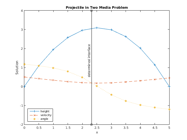
Example
This example intends to illustrate the use of the break-point and equation solving facilities of
nag_ode_bvp_shoot_genpar_algeq (d02sa). Most of the facilities which are common to
nag_ode_bvp_shoot_genpar_algeq (d02sa) and
nag_ode_bvp_shoot_genpar (d02hb) are illustrated in the example in the specification of
nag_ode_bvp_shoot_genpar (d02hb) (which should also be consulted).
The program solves a projectile problem in two media determining the position of change of media, , and the gravity and viscosity in the second medium ( represents gravity and represents viscosity).
Open in the MATLAB editor:
d02sa_example
function d02sa_example
fprintf('d02sa example results\n\n');
global ykeep ncall xkeep;
p = [1.2; 0.032; 2.5;0.2];
n1 = int64(3);
pe = [0.001; 0.001; 0.001; 0.001];
pf = [1e-06; 1e-06; 1e-06; 1e-06];
e = [1e-05; 1e-05; 1e-05];
dp = [0; 0; 0; 0];
swp = zeros(3, 6);
icount = int64(0);
ymax = 0;
ncall = 0;
ykeep = zeros(1,3);
xkeep = zeros(1,1);
fprintf(' x y(1) y(2) y(3)\n')
[p, pf, dp, swp, w, ifail] = ...
d02sa(...
p, n1, pe, pf, e, dp, swp, icount, @range, @bc, @fcn, ...
@eqn, @constr, ymax, @monit, @prsol);
fig1 = figure;
display_plot(xkeep,ykeep)
function z = prsol(z, y, n)
global ykeep ncall xkeep;
ncall = ncall+1;
fprintf(' %6.4f',z);
xkeep(ncall,1) = z;
fprintf('%10.4f ', y(1:n));
fprintf('\n');
z = z+0.5;
if (abs(z-5) < 0.25)
z = 5;
end
ykeep(ncall,:) = y;
function x = range(npoint, p, m)
x = zeros(npoint,1);
x(1) = 0;
x(2) = p(3);
x(3) = 5;
function [g1, g2] = bc(p, m, n)
g1 = [0, 0.5, p(1)];
g2 = [0, 0.45, -1.2];
function f = fcn(x, y, n, p, m, interval)
f = zeros(n,1);
f(1) = tan(y(3));
if (interval == 1)
f(2) = -0.032d0*tan(y(3))/y(2) - 0.02d0*y(2)/cos(y(3));
f(3) = -0.032d0/y(2)^2;
else
f(2) = -p(2)*tan(y(3))/y(2) - p(4)*y(2)/cos(y(3));
f(3) = -p(2)/y(2)^2;
end
function eq = eqn(q,p,m)
eq = zeros(q,1);
eq(1) = 0.02 - p(4) - 1.0d-5*p(3);
function result = constr(p,n)
result = true;
for i=1:n
if p(i) < 0
result = false;
end
end
if p(3) > 5
result = false;
end
function monit(istate, iflag, ifail1, p, m, f, pnorm, pnorm1, eps, d)
function display_plot(xkeep,ykeep)
plot(xkeep, ykeep(:,1), '-+', ...
xkeep, ykeep(:,2), '--x', ...
xkeep, ykeep(:,3), ':*');
title('Projectile in Two Media Problem');
xlabel('x');
ylabel('Solution');
legend('height','velocity','angle','Location','SouthWest');
xmin = min(xkeep);
xmax = max(xkeep);
ymin = round(min(min(ykeep))-1);
ymax = round(max(max(ykeep))+1);
axis([xmin xmax ymin ymax]);
stem(xkeep, ykeep, ymin, ymax, 'determined interface');
function stem(x, y, ymin, ymax, label)
for i = 1:length(x)
if y(i,2) > y(i,3)
break
end
end
m(1:2) = (y(i,2:3) - y(i-1,2:3))/(x(i)-x(i-1));
c(1:2) = y(i,2:3) - m(1:2)*x(i);
xx = (c(2)-c(1))/(m(1)-m(2));
hold on
plot([xx,xx],[ymin,ymax],'k-s');
text('Position', [xx-0.1,0.5], 'String', label, 'Rotation', 90.0)
d02sa example results

   x        y(1)        y(2)        y(3)
 0.0000    0.0000      0.5000      1.1753
 0.5000    1.0881      0.4127      1.0977
 1.0000    1.9501      0.3310      0.9802
 1.5000    2.5768      0.2582      0.7918
 2.0000    2.9606      0.2019      0.4796
 2.5000    3.0958      0.1773      0.0245
 3.0000    2.9861      0.1935     -0.4353
 3.5000    2.6289      0.2409     -0.7679
 4.0000    2.0181      0.3047     -0.9767
 4.5000    1.1454      0.3759     -1.1099
 5.0000   -0.0000      0.4500     -1.2000
PDF version (NAG web site
, 64-bit version, 64-bit version)
© The Numerical Algorithms Group Ltd, Oxford, UK. 2009–2015