hide long namesshow long names
hide short namesshow short names
Integer type:  int32  int64  nag_int  show int32  show int32  show int64  show int64  show nag_int  show nag_int

PDF version (NAG web site, 64-bit version, 64-bit version)
Chapter Contents
Chapter Introduction
NAG Toolbox

NAG Toolbox: nag_ode_bvp_coll_nlin_contin (d02tx)

 Contents

    1  Purpose
    2  Syntax
    7  Accuracy
    9  Example

Purpose

nag_ode_bvp_coll_nlin_contin (d02tx) allows a solution to a nonlinear two-point boundary value problem computed by nag_ode_bvp_coll_nlin_solve (d02tl) to be used as an initial approximation in the solution of a related nonlinear two-point boundary value problem in a continuation call to nag_ode_bvp_coll_nlin_solve (d02tl).

Syntax

[rcomm, icomm, ifail] = d02tx(nmesh, mesh, ipmesh, rcomm, icomm, 'mxmesh', mxmesh)
[rcomm, icomm, ifail] = nag_ode_bvp_coll_nlin_contin(nmesh, mesh, ipmesh, rcomm, icomm, 'mxmesh', mxmesh)

Description

nag_ode_bvp_coll_nlin_contin (d02tx) and its associated functions (nag_ode_bvp_coll_nlin_solve (d02tl), nag_ode_bvp_coll_nlin_setup (d02tv), nag_ode_bvp_coll_nlin_interp (d02ty) and nag_ode_bvp_coll_nlin_diag (d02tz)) solve the two-point boundary value problem for a nonlinear system of ordinary differential equations
y1m1 x = f1 x,y1,y11,,y1m1-1,y2,,ynmn-1 y2m2 x = f2 x,y1,y11,,y1m1-1,y2,,ynmn-1 ynmn x = fn x,y1,y11,,y1m1-1,y2,,ynmn-1  
over an interval a,b subject to p (>0) nonlinear boundary conditions at a and q (>0) nonlinear boundary conditions at b, where p+q = i=1 n mi . Note that yi m x is the mth derivative of the ith solution component. Hence yi 0 x=yix. The left boundary conditions at a are defined as
gizya=0,  i=1,2,,p,  
and the right boundary conditions at b as
g-jzyb=0,  j=1,2,,q,  
where y=y1,y2,,yn and
zyx = y1x, y11 x ,, y1m1-1 x ,y2x,, ynmn-1 x .  
First, nag_ode_bvp_coll_nlin_setup (d02tv) must be called to specify the initial mesh, error requirements and other details. Then, nag_ode_bvp_coll_nlin_solve (d02tl) can be used to solve the boundary value problem. After successful computation, nag_ode_bvp_coll_nlin_diag (d02tz) can be used to ascertain details about the final mesh. nag_ode_bvp_coll_nlin_interp (d02ty) can be used to compute the approximate solution anywhere on the interval a,b using interpolation.
If the boundary value problem being solved is one of a sequence of related problems, for example as part of some continuation process, then nag_ode_bvp_coll_nlin_contin (d02tx) should be used between calls to nag_ode_bvp_coll_nlin_solve (d02tl). This avoids the overhead of a complete initialization when the setup function nag_ode_bvp_coll_nlin_setup (d02tv) is used. nag_ode_bvp_coll_nlin_contin (d02tx) allows the solution values computed in the previous call to nag_ode_bvp_coll_nlin_solve (d02tl) to be used as an initial approximation for the solution in the next call to nag_ode_bvp_coll_nlin_solve (d02tl).
You must specify the new initial mesh. The previous mesh can be obtained by a call to nag_ode_bvp_coll_nlin_diag (d02tz). It may be used unchanged as the new mesh, in which case any fixed points in the previous mesh remain as fixed points in the new mesh. Fixed and other points may be added or subtracted from the mesh by manipulation of the contents of the array argument ipmesh. Initial values for the solution components on the new mesh are computed by interpolation on the values for the solution components on the previous mesh.
The functions are based on modified versions of the codes COLSYS and COLNEW (see Ascher et al. (1979) and Ascher and Bader (1987)). A comprehensive treatment of the numerical solution of boundary value problems can be found in Ascher et al. (1988) and Keller (1992).

References

Ascher U M and Bader G (1987) A new basis implementation for a mixed order boundary value ODE solver SIAM J. Sci. Stat. Comput. 8 483–500
Ascher U M, Christiansen J and Russell R D (1979) A collocation solver for mixed order systems of boundary value problems Math. Comput. 33 659–679
Ascher U M, Mattheij R M M and Russell R D (1988) Numerical Solution of Boundary Value Problems for Ordinary Differential Equations Prentice–Hall
Keller H B (1992) Numerical Methods for Two-point Boundary-value Problems Dover, New York

Parameters

Compulsory Input Parameters

1:     nmesh int64int32nag_int scalar
Suggested value: n*+1/2, where n* is the number of mesh points used in the previous mesh as returned in the argument nmesh of nag_ode_bvp_coll_nlin_diag (d02tz).
The number of points to be used in the new initial mesh. It is strongly recommended that if this function is called that the suggested value (see below) for nmesh is used. In this case the arrays mesh and ipmesh returned by nag_ode_bvp_coll_nlin_diag (d02tz) can be passed to this function without any modification.
Constraint: 6nmeshmxmesh+1/2.
2:     meshmxmesh – double array
Suggested value: the argument mesh returned from a call to nag_ode_bvp_coll_nlin_diag (d02tz).
The nmesh points to be used in the new initial mesh as specified by ipmesh.
Constraint: meshij < meshij+1, for j=1,2,,nmesh-1, the values of i1,i2,,inmesh are defined in ipmesh.
meshi1 must contain the left boundary point, a, and meshinmesh must contain the right boundary point, b, as specified in the previous call to nag_ode_bvp_coll_nlin_setup (d02tv).
3:     ipmeshmxmesh int64int32nag_int array
Suggested value: the argument ipmesh returned in a call to nag_ode_bvp_coll_nlin_diag (d02tz).
Specifies the points in mesh to be used as the new initial mesh. Let ij:j=1,2,,nmesh be the set of array indices of ipmesh such that ipmeshij=1​ or ​2 and 1=i1<i2<<inmesh. Then meshij will be included in the new initial mesh.
If ipmeshij=1, meshij will be a fixed point in the new initial mesh.
If ipmeshk=3 for any k, then meshk will not be included in the new mesh.
Constraints:
  • ipmeshk=1, 2 or 3, for k=1,2,,inmesh;
  • ipmesh1=ipmeshinmesh=1.
4:     rcomm* – double array
Note: the dimension of this array is dictated by the requirements of associated functions that must have been previously called. This array must be the same array passed as argument rcomm in the previous call to nag_ode_bvp_coll_nlin_solve (d02tl).
This must be the same array as supplied to nag_ode_bvp_coll_nlin_solve (d02tl) and must remain unchanged between calls.
5:     icomm* int64int32nag_int array
Note: the dimension of this array is dictated by the requirements of associated functions that must have been previously called. This array must be the same array passed as argument icomm in the previous call to nag_ode_bvp_coll_nlin_solve (d02tl).
This must be the same array as supplied to nag_ode_bvp_coll_nlin_solve (d02tl) and must remain unchanged between calls.

Optional Input Parameters

1:     mxmesh int64int32nag_int scalar
Default: the dimension of the arrays mesh, ipmesh. (An error is raised if these dimensions are not equal.)
The maximum number of points allowed in the mesh.
Constraint: this must be identical to the value supplied for the argument mxmesh in the prior call to nag_ode_bvp_coll_nlin_setup (d02tv).

Output Parameters

1:     rcomm* – double array
Note: the dimension of this array is dictated by the requirements of associated functions that must have been previously called. This array must be the same array passed as argument rcomm in the previous call to nag_ode_bvp_coll_nlin_solve (d02tl).
Contains information about the solution for use on subsequent calls to associated functions.
2:     icomm* int64int32nag_int array
Note: the dimension of this array is dictated by the requirements of associated functions that must have been previously called. This array must be the same array passed as argument icomm in the previous call to nag_ode_bvp_coll_nlin_solve (d02tl).
Contains information about the solution for use on subsequent calls to associated functions.
3:     ifail int64int32nag_int scalar
ifail=0 unless the function detects an error (see Error Indicators and Warnings).

Error Indicators and Warnings

Errors or warnings detected by the function:
   ifail=1
An element of ipmesh was set to -1 before nmesh elements containing 1 or 2 were detected.
Constraint: ipmesh1=1.
Constraint: mxmesh=mxmesh in nag_ode_bvp_coll_nlin_setup (d02tv).
Constraint: nmeshmxmesh+1/2.
Constraint: nmesh6.
Expected _ elements of ipmesh to be 1 or 2, but _ such elements found.
ipmeshi-1, 1, 2 or 3 for some i.
The entries in mesh are not strictly increasing.
The first element of array mesh does not coincide with the left hand end of the range previously specified.
The last point of the new mesh does not coincide with the right hand end of the range previously specified.
The solver function did not produce any results suitable for remeshing.
The solver function does not appear to have been called.
You have set the element of ipmesh corresponding to the last element of mesh to be included in the new mesh as _, which is not 1.
   ifail=-99
An unexpected error has been triggered by this routine. Please contact NAG.
   ifail=-399
Your licence key may have expired or may not have been installed correctly.
   ifail=-999
Dynamic memory allocation failed.

Accuracy

Not applicable.

Further Comments

For problems where sharp changes of behaviour are expected over short intervals it may be advisable to:
cluster the mesh points where sharp changes in behaviour are expected;
maintain fixed points in the mesh using the argument ipmesh to ensure that the remeshing process does not inadvertently remove mesh points from areas of known interest.
In the absence of any other information about the expected behaviour of the solution, using the values suggested in Arguments for nmesh, ipmesh and mesh is strongly recommended.

Example

This example illustrates the use of continuation, solution on an infinite range, and solution of a system of two differential equations of orders 3 and 2. See also nag_ode_bvp_coll_nlin_solve (d02tl), nag_ode_bvp_coll_nlin_setup (d02tv), nag_ode_bvp_coll_nlin_interp (d02ty) and nag_ode_bvp_coll_nlin_diag (d02tz), for the illustration of other facilities.
Consider the problem of swirling flow over an infinite stationary disk with a magnetic field along the axis of rotation. See Ascher et al. (1988) and the references therein. After transforming from a cylindrical coordinate system r,θ,z, in which the θ component of the corresponding velocity field behaves like r-n, the governing equations are
f+123-nff+n f 2+g2-sf = γ2 g+123-nfg+n-1gf-sg-1 = 0  
with boundary conditions
f0=f0=g0= 0,   f= 0,   g=γ,  
where s is the magnetic field strength, and γ is the Rossby number.
Some solutions of interest are for γ=1, small n and s0. An added complication is the infinite range, which we approximate by 0,L. We choose n=0.2 and first solve for L=60.0,s=0.24 using the initial approximations fx=-x2e-x and gx=1.0-e-x, which satisfy the boundary conditions, on a uniform mesh of 21 points. Simple continuation on the parameters L and s using the values L=120.0,s=0.144 and then L=240.0,s=0.0864 is used to compute further solutions. We use the suggested values for nmesh, ipmesh and mesh in the call to nag_ode_bvp_coll_nlin_contin (d02tx) prior to a continuation call, that is only every second point of the preceding mesh is used.
The equations are first mapped onto 0,1 to yield
f = L3γ2-g2+L2sg-L123-nff+n g 2 g = L2sg-1-L123-nfg+n-1fg.  
function d02tx_example


fprintf('d02tx example results\n\n');

global en s el; % For communication with local functions

% Initialize variables and arrays.
neq  = int64(2);
nlbc = int64(3);
nrbc = int64(2);
ncol = int64(6);
mmax = int64(3);
m    = int64([3; 2]);
tols = [0.00001; 0.00001];

% Set values for problem-specific physical parameters.
el = 60;
s  = 0.24;
en = 0.2;

% Set up the mesh.
nmesh  = int64(21);
mxmesh = int64(250);
mesh = zeros(mxmesh,1);
ipmesh = zeros(mxmesh,1,'int64');

% Set initial mesh with constant spacing.
dx = 1/double(nmesh-1);
mesh(1:nmesh) = [0:dx:1];

% Specify mesh end points as fixed.
ipmesh(1)         = 1;
ipmesh(2:nmesh-1) = 2;
ipmesh(nmesh)     = 1;

% Prepare to store results for plotting.
xarray = zeros(1,1);
yarray1 = zeros(1,1);
yarray2 = zeros(1,1);

% d02tv is a setup routine to be called prior to d02tk.
[work, iwork, ifail] = d02tv(...
                              m, nlbc, nrbc, ncol, tols, nmesh, mesh, ipmesh);

ncont = 3;

% We run through the calculation three times with different parameter sets.
for jcont = 1:ncont
  fprintf('\n Tolerance = %8.1e, L = %8.3f, S = %6.4f\n\n', tols(1), el, s);
  
  % Call d02tk to solve BVP for this set of parameters.
  [work, iwork, ifail] = d02tk(...
                               @ffun, @fjac, @gafun, @gbfun, @gajac, ...
                               @gbjac, @guess, work, iwork);

  % Call d02tz to extract mesh from solution.
  [nmesh, mesh, ipmesh, ermx, iermx, ijermx, ifail] = ...
  d02tz( ...
        mxmesh, work, iwork);

  % Output mesh results.
  fprintf(' Used a mesh of %d points\n', nmesh);
  fprintf(' Maximum error = %10.2e in interval %d for component %d\n\n',...
          ermx, iermx, ijermx);

  % Output solution, and store it for plotting.
  fprintf(' Solution on original interval:\n');
  fprintf('    x          f           g\n');
  for i=1:16
    xx = double(i-1)*2/el;

    % Call d02ty to perform interpolation on the solution.
    [y, work, ifail] = d02ty(...
                              xx, neq, mmax, work, iwork);
    fprintf(' %6.2f    %8.4f    %8.4f\n', xx*el, y(1,1), y(2,1));
    xarray(i) = xx*el;
    yarray1(i) = y(1,1);
    yarray2(i) = y(2,1);
  end
  for i=1:10
    xx = (30+(el-30)*double(i)/10)/el;

    [y, work, ifail] = d02ty(...
                             xx, neq, mmax, work, iwork);
    fprintf(' %6.2f    %8.4f    %8.4f\n', xx*el, y(1,1), y(2,1));
    xarray(i+16) = xx*el;
    yarray1(i+16) = y(1,1);
    yarray2(i+16) = y(2,1);
  end

  % Plot results for this parameter set.
  if (jcont==1)
    fig1 = figure;
  elseif (jcont==2)
    fig2 = figure;
  else
    fig3 = figure;
  end    
  display_plot(xarray, yarray1, yarray2, el, s)

  % Select mesh for next calculation.
  if jcont < ncont
    el = 2*el;
    s = 0.6*s;
    nmesh = (nmesh+1)/2;

    % d02tx allows the current solution to be used as an initial
    % approximation to the solution of a related problem.
    [work, iwork, ifail] = d02tx(...
                                  nmesh, mesh, ipmesh, work, iwork);
  end
end


function [f] = ffun(x, y, neq, m)
  % Evaluate derivative functions (rhs of system of ODEs).

  global en s el
  f = zeros(neq, 1);
  f(1) = el^3*(1-y(2,1)^2) + el^2*s*y(1,2) - ...
         el*(0.5*(3-en)*y(1,1)*y(1,3) + en*y(1,2)^2);
  f(2) = el^2*s*(y(2,1)-1) - ...
         el*(0.5*(3-en)*y(1,1)*y(2,2) + (en-1)*y(1,2)*y(2,1));

function [dfdy] = fjac(x, y, neq, m)
  % Evaluate Jacobians (partial derivatives of f).
         
  global en s el
  dfdy = zeros(neq, neq, 3);
  dfdy(1,2,1) = -2*el^3*y(2,1);
  dfdy(1,1,1) = -el*0.5*(3-en)*y(1,3);
  dfdy(1,1,2) = el^2*s - el*2*en*y(1,2);
  dfdy(1,1,3) = -el*0.5*(3-en)*y(1,1);
  dfdy(2,2,1) = el^2*s - el*(en-1)*y(1,2);
  dfdy(2,2,2) = -el*0.5*(3-en)*y(1,1);
  dfdy(2,1,1) = -el*0.5*(3-en)*y(2,2);
  dfdy(2,1,2) = -el*(en-1)*y(2,1);

function [ga] = gafun(ya, neq, m, nlbc)
  % Evaluate boundary conditions at left-hand end of range.

  global en s el
  ga = zeros(nlbc, 1);
  ga(1) = ya(1,1);
  ga(2) = ya(1,2);
  ga(3) = ya(2,1);

function [dgady] = gajac(ya, neq, m, nlbc)
  % Evaluate Jacobians (partial derivatives of ga).

  global en s el
  dgady = zeros(nlbc, neq, 3);
  dgady(1,1,1) = 1;
  dgady(2,1,2) = 1;
  dgady(3,2,1) = 1;

function [gb] = gbfun(yb, neq, m, nrbc)
  % Evaluate boundary conditions at right-hand end of range.

  global en s el
  gb = zeros(nrbc, 1);
  gb(1) = yb(1,2);
  gb(2) = yb(2,1) - 1;

function [dgbdy] = gbjac(yb, neq, m, nrbc)
  % Evaluate Jacobians (partial derivatives of gb).

  global en s el
  dgbdy = zeros(nrbc, neq, 3);
  dgbdy(1,1,2) = 1;
  dgbdy(2,2,1) = 1;

function [y, dym] = guess(x, neq, m)
  % Evaluate initial approximations to solution components and derivatives.

  global en s el
  y = zeros(neq, 3);
  dym = zeros(neq, 1);
  ex = x*el;
  expmx = exp(-ex);
  y(1,1) = -ex^2*expmx;
  y(1,2) = (-2*ex+ex^2)*expmx;
  y(1,3) = (-2+4*ex-ex^2)*expmx;
  y(2,1) = 1 - expmx;
  y(2,2) = expmx;
  dym(1) = (6-6*ex+ex^2)*expmx;
  dym(2) = -expmx;

function display_plot(xarray,yarray1,yarray2,el,s)
  % Formatting for title and axis labels.
  % Plot the results.
  plot(xarray, yarray1, '-+', xarray, yarray2, '--x');
  % Add title.
  title({['Swirling Flow over Disc in Axial Magnetic Field '], ...
         ['with L = ',num2str(el), ' and s = ',num2str(s)]})
  % Label the axes.
  xlabel('Radial Distance from Magnetic Field');
  ylabel('Velocities');
  % Add a legend.
  legend('axial velocity','tangential velocity','Location','Best')
d02tx example results


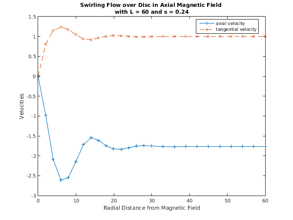
 Tolerance =  1.0e-05, L =   60.000, S = 0.2400

 Used a mesh of 21 points
 Maximum error =   2.66e-08 in interval 7 for component 1

 Solution on original interval:
    x          f           g
   0.00      0.0000      0.0000
   2.00     -0.9769      0.8011
   4.00     -2.0900      1.1459
   6.00     -2.6093      1.2389
   8.00     -2.5498      1.1794
  10.00     -2.1397      1.0478
  12.00     -1.7176      0.9395
  14.00     -1.5465      0.9206
  16.00     -1.6127      0.9630
  18.00     -1.7466      1.0068
  20.00     -1.8286      1.0244
  22.00     -1.8338      1.0185
  24.00     -1.7956      1.0041
  26.00     -1.7582      0.9940
  28.00     -1.7445      0.9926
  30.00     -1.7515      0.9965
  33.00     -1.7695      1.0019
  36.00     -1.7730      1.0018
  39.00     -1.7673      0.9998
  42.00     -1.7645      0.9993
  45.00     -1.7659      0.9999
  48.00     -1.7672      1.0002
  51.00     -1.7671      1.0001
  54.00     -1.7666      0.9999
  57.00     -1.7665      0.9999
  60.00     -1.7666      1.0000

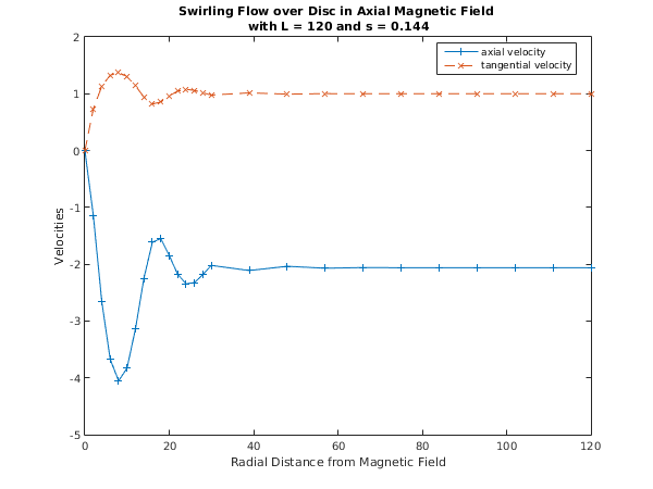
 Tolerance =  1.0e-05, L =  120.000, S = 0.1440

 Used a mesh of 21 points
 Maximum error =   6.88e-06 in interval 7 for component 2

 Solution on original interval:
    x          f           g
   0.00      0.0000      0.0000
   2.00     -1.1406      0.7317
   4.00     -2.6531      1.1315
   6.00     -3.6721      1.3250
   8.00     -4.0539      1.3707
  10.00     -3.8285      1.3003
  12.00     -3.1339      1.1407
  14.00     -2.2469      0.9424
  16.00     -1.6146      0.8201
  18.00     -1.5472      0.8549
  20.00     -1.8483      0.9623
  22.00     -2.1761      1.0471
  24.00     -2.3451      1.0778
  26.00     -2.3236      1.0600
  28.00     -2.1784      1.0165
  30.00     -2.0214      0.9775
  39.00     -2.1109      1.0155
  48.00     -2.0362      0.9931
  57.00     -2.0709      1.0023
  66.00     -2.0588      0.9995
  75.00     -2.0616      1.0000
  84.00     -2.0615      1.0001
  93.00     -2.0611      0.9999
 102.00     -2.0614      1.0000
 111.00     -2.0613      1.0000
 120.00     -2.0613      1.0000

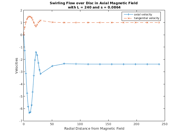
 Tolerance =  1.0e-05, L =  240.000, S = 0.0864

 Used a mesh of 81 points
 Maximum error =   3.30e-07 in interval 19 for component 2

 Solution on original interval:
    x          f           g
   0.00      0.0000      0.0000
   2.00     -1.2756      0.6404
   4.00     -3.1604      1.0463
   6.00     -4.7459      1.3011
   8.00     -5.8265      1.4467
  10.00     -6.3412      1.5036
  12.00     -6.2862      1.4824
  14.00     -5.6976      1.3886
  16.00     -4.6568      1.2263
  18.00     -3.3226      1.0042
  20.00     -2.0328      0.7718
  22.00     -1.4035      0.6943
  24.00     -1.6603      0.8218
  26.00     -2.2975      0.9928
  28.00     -2.8661      1.1139
  30.00     -3.1641      1.1641
  51.00     -2.5307      1.0279
  72.00     -2.3520      0.9919
  93.00     -2.3674      0.9975
 114.00     -2.3799      1.0003
 135.00     -2.3800      1.0002
 156.00     -2.3792      1.0000
 177.00     -2.3791      1.0000
 198.00     -2.3792      1.0000
 219.00     -2.3792      1.0000
 240.00     -2.3792      1.0000
d02tx_fig1.png
d02tx_fig2.png
d02tx_fig3.png

PDF version (NAG web site, 64-bit version, 64-bit version)
Chapter Contents
Chapter Introduction
NAG Toolbox

© The Numerical Algorithms Group Ltd, Oxford, UK. 2009–2015