PDF version (NAG web site
, 64-bit version, 64-bit version)
NAG Toolbox: nag_fit_1dspline_auto (e02be)
Purpose
nag_fit_1dspline_auto (e02be) computes a cubic spline approximation to an arbitrary set of data points. The knots of the spline are located automatically, but a single argument must be specified to control the trade-off between closeness of fit and smoothness of fit.
Syntax
[
n,
lamda,
c,
fp,
wrk,
iwrk,
ifail] = e02be(
start,
x,
y,
w,
s,
n,
lamda,
wrk,
iwrk, 'm',
m, 'nest',
nest)
[
n,
lamda,
c,
fp,
wrk,
iwrk,
ifail] = nag_fit_1dspline_auto(
start,
x,
y,
w,
s,
n,
lamda,
wrk,
iwrk, 'm',
m, 'nest',
nest)
Note: the interface to this routine has changed since earlier releases of the toolbox:
| At Mark 22: |
lwrk was removed from the interface |
Description
nag_fit_1dspline_auto (e02be) determines a smooth cubic spline approximation to the set of data points , with weights , for .
The spline is given in the B-spline representation
where
denotes the normalized cubic B-spline defined upon the knots
.
The total number of these knots and their values are chosen automatically by the function. The knots are the interior knots; they divide the approximation interval into sub-intervals. The coefficients are then determined as the solution of the following constrained minimization problem:
minimize
subject to the constraint
| where |
|
stands for the discontinuity jump in the third order derivative of at the interior knot , |
| |
|
denotes the weighted residual , |
| and |
|
is a non-negative number to be specified by you. |
The quantity
can be seen as a measure of the (lack of) smoothness of
, while closeness of fit is measured through
. By means of the argument
, ‘the smoothing factor’, you can then control the balance between these two (usually conflicting) properties. If
is too large, the spline will be too smooth and signal will be lost (underfit); if
is too small, the spline will pick up too much noise (overfit). In the extreme cases the function will return an interpolating spline
if
is set to zero, and the weighted least squares cubic polynomial
if
is set very large. Experimenting with
values between these two extremes should result in a good compromise. (See
Choice of
for advice on choice of
.)
The method employed is outlined in
Outline of Method Used and fully described in
Dierckx (1975),
Dierckx (1981) and
Dierckx (1982). It involves an adaptive strategy for locating the knots of the cubic spline (depending on the function underlying the data and on the value of
), and an iterative method for solving the constrained minimization problem once the knots have been determined.
Values of the computed spline, or of its derivatives or definite integral, can subsequently be computed by calling
nag_fit_1dspline_eval (e02bb),
nag_fit_1dspline_deriv (e02bc) or
nag_fit_1dspline_integ (e02bd), as described in
Evaluation of Computed Spline.
References
Dierckx P (1975) An algorithm for smoothing, differentiating and integration of experimental data using spline functions J. Comput. Appl. Math. 1 165–184
Dierckx P (1981) An improved algorithm for curve fitting with spline functions Report TW54 Department of Computer Science, Katholieke Univerciteit Leuven
Dierckx P (1982) A fast algorithm for smoothing data on a rectangular grid while using spline functions SIAM J. Numer. Anal. 19 1286–1304
Reinsch C H (1967) Smoothing by spline functions Numer. Math. 10 177–183
Parameters
Compulsory Input Parameters
- 1:
– string (length ≥ 1)
-
Must be set to 'C' or 'W'.
- The function will build up the knot set starting with no interior knots. No values need be assigned to the arguments n, lamda, wrk or iwrk.
- The function will restart the knot-placing strategy using the knots found in a previous call of the function. In this case, the arguments n, lamda, wrk, and iwrk must be unchanged from that previous call. This warm start can save much time in searching for a satisfactory value of .
Constraint:
or .
- 2:
– double array
-
The values
of the independent variable (abscissa) , for .
Constraint:
.
- 3:
– double array
-
The values
of the dependent variable (ordinate) , for .
- 4:
– double array
-
The values
of the weights, for
. For advice on the choice of weights, see
Weighting of data points in the E02 Chapter Introduction.
Constraint:
, for .
- 5:
– double scalar
-
The smoothing factor,
.
If , the function returns an interpolating spline.
If
is smaller than
machine precision, it is assumed equal to zero.
For advice on the choice of
, see
Description and
Choice of
.
Constraint:
.
- 6:
– int64int32nag_int scalar
-
If the warm start option is used, the value of
n must be left unchanged from the previous call.
- 7:
– double array
-
If the warm start option is used, the values must be left unchanged from the previous call.
- 8:
– double array
-
lwrk, the dimension of the array, must satisfy the constraint
.
If the warm start option is used on entry, the values must be left unchanged from the previous call.
- 9:
– int64int32nag_int array
-
If the warm start option is used, on entry, the values must be left unchanged from the previous call.
This array is used as workspace.
Optional Input Parameters
- 1:
– int64int32nag_int scalar
-
Default:
the dimension of the arrays
x,
y,
w. (An error is raised if these dimensions are not equal.)
, the number of data points.
Constraint:
.
- 2:
– int64int32nag_int scalar
-
Default:
the dimension of the arrays
lamda,
iwrk. (An error is raised if these dimensions are not equal.)
An overestimate for the number, , of knots required.
Constraint:
. In most practical situations,
is sufficient.
nest never needs to be larger than
, the number of knots needed for interpolation
.
Output Parameters
- 1:
– int64int32nag_int scalar
-
The total number, , of knots of the computed spline.
- 2:
– double array
-
The knots of the spline, i.e., the positions of the interior knots
as well as the positions of the additional knots
and
needed for the B-spline representation.
- 3:
– double array
-
The coefficient
of the B-spline in the spline approximation , for .
- 4:
– double scalar
-
The sum of the squared weighted residuals,
, of the computed spline approximation. If
, this is an interpolating spline.
fp should equal
within a relative tolerance of
unless
when the spline has no interior knots and so is simply a cubic polynomial. For knots to be inserted,
must be set to a value below the value of
fp produced in this case.
- 5:
– double array
-
- 6:
– int64int32nag_int array
-
This array is used as workspace.
- 7:
– int64int32nag_int scalar
unless the function detects an error (see
Error Indicators and Warnings).
Error Indicators and Warnings
Errors or warnings detected by the function:
-
-
| On entry, | or , |
| or | , |
| or | , |
| or | and , |
| or | , |
| or | . |
-
-
The weights are not all strictly positive.
-
-
The values of , for , are not in strictly increasing order.
-
-
The number of knots required is greater than
nest. Try increasing
nest and, if necessary, supplying larger arrays for the arguments
lamda,
c,
wrk and
iwrk. However, if
nest is already large, say
, then this error exit may indicate that
s is too small.
-
-
The iterative process used to compute the coefficients of the approximating spline has failed to converge. This error exit may occur if
s has been set very small. If the error persists with increased
s, contact
NAG.
-
An unexpected error has been triggered by this routine. Please
contact
NAG.
-
Your licence key may have expired or may not have been installed correctly.
-
Dynamic memory allocation failed.
If
or
, a spline approximation is returned, but it fails to satisfy the fitting criterion (see
(2) and
(3)) – perhaps by only a small amount, however.
Accuracy
On successful exit, the approximation returned is such that its weighted sum of squared residuals
(as in
(3)) is equal to the smoothing factor
, up to a specified relative tolerance of
– except that if
,
may be significantly less than
: in this case the computed spline is simply a weighted least squares polynomial approximation of degree
, i.e., a spline with no interior knots.
Further Comments
Timing
The time taken for a call of nag_fit_1dspline_auto (e02be) depends on the complexity of the shape of the data, the value of the smoothing factor , and the number of data points. If nag_fit_1dspline_auto (e02be) is to be called for different values of , much time can be saved by setting after the first call.
Choice of S
If the weights have been correctly chosen (see
Weighting of data points in the E02 Chapter Introduction), the standard deviation of
would be the same for all
, equal to
, say. In this case, choosing the smoothing factor
in the range
, as suggested by
Reinsch (1967), is likely to give a good start in the search for a satisfactory value. Otherwise, experimenting with different values of
will be required from the start, taking account of the remarks in
Description.
In that case, in view of computation time and memory requirements, it is recommended to start with a very large value for
and so determine the least squares cubic polynomial; the value returned in
fp, call it
, gives an upper bound for
. Then progressively decrease the value of
to obtain closer fits – say by a factor of
in the beginning, i.e.,
,
, and so on, and more carefully as the approximation shows more details.
The number of knots of the spline returned, and their location, generally depend on the value of and on the behaviour of the function underlying the data. However, if nag_fit_1dspline_auto (e02be) is called with , the knots returned may also depend on the smoothing factors of the previous calls. Therefore if, after a number of trials with different values of and , a fit can finally be accepted as satisfactory, it may be worthwhile to call nag_fit_1dspline_auto (e02be) once more with the selected value for but now using . Often, nag_fit_1dspline_auto (e02be) then returns an approximation with the same quality of fit but with fewer knots, which is therefore better if data reduction is also important.
Outline of Method Used
If
, the requisite number of knots is known in advance, i.e.,
; the interior knots are located immediately as
, for
. The corresponding least squares spline (see
nag_fit_1dspline_knots (e02ba)) is then an interpolating spline and therefore a solution of the problem.
If
, a suitable knot set is built up in stages (starting with no interior knots in the case of a cold start but with the knot set found in a previous call if a warm start is chosen). At each stage, a spline is fitted to the data by least squares (see
nag_fit_1dspline_knots (e02ba)) and
, the weighted sum of squares of residuals, is computed. If
, new knots are added to the knot set to reduce
at the next stage. The new knots are located in intervals where the fit is particularly poor, their number depending on the value of
and on the progress made so far in reducing
. Sooner or later, we find that
and at that point the knot set is accepted. The function then goes on to compute the (unique) spline which has this knot set and which satisfies the full fitting criterion specified by
(2) and
(3). The theoretical solution has
. The function computes the spline by an iterative scheme which is ended when
within a relative tolerance of
. The main part of each iteration consists of a linear least squares computation of special form, done in a similarly stable and efficient manner as in
nag_fit_1dspline_knots (e02ba).
An exception occurs when the function finds at the start that, even with no interior knots , the least squares spline already has its weighted sum of squares of residuals . In this case, since this spline (which is simply a cubic polynomial) also has an optimal value for the smoothness measure , namely zero, it is returned at once as the (trivial) solution. It will usually mean that has been chosen too large.
For further details of the algorithm and its use, see
Dierckx (1981).
Evaluation of Computed Spline
The value of the computed spline at a given value
x may be obtained in the double variable
s by the call:
[s, ifail] = e02bb(lamda, c, x);
where
n,
lamda and
c are the output arguments of
nag_fit_1dspline_auto (e02be).
The values of the spline and its first three derivatives at a given value
x may be obtained in the double array
s of dimension at least
by the call:
[s, ifail] = e02bc(lamda, c, x, left);
where if
, left-hand derivatives are computed and if
, right-hand derivatives are calculated. The value of
left is only relevant if
x is an interior knot (see
nag_fit_1dspline_deriv (e02bc)).
The value of the definite integral of the spline over the interval
to
can be obtained in the double variable
dint by the call:
[dint, ifail] = e02bd(lamda, c);
(see
nag_fit_1dspline_integ (e02bd)).
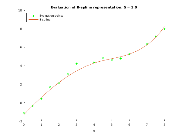
Example
This example reads in a set of data values, followed by a set of values of . For each value of it calls nag_fit_1dspline_auto (e02be) to compute a spline approximation, and prints the values of the knots and the B-spline coefficients .
The program includes code to evaluate the computed splines, by calls to
nag_fit_1dspline_eval (e02bb), at the points
and at points mid-way between them. These values are not printed out, however; instead the results are illustrated by plots of the computed splines, together with the data points (indicated by
) and the positions of the knots (indicated by vertical lines): the effect of decreasing
can be clearly seen.
Open in the MATLAB editor:
e02be_example
function e02be_example
fprintf('e02be example results\n\n');
start = 'C';
data = [0.0 -1.100 1.0;
0.5 -0.372 2.0;
1.0 0.431 1.5;
1.5 1.690 1.0;
2.0 2.110 3.0;
2.5 3.100 1.0;
3.0 4.230 0.5;
4.0 4.350 1.0;
4.5 4.810 2.0;
5.0 4.610 2.5;
5.5 4.790 1.0;
6.0 5.230 3.0;
7.0 6.350 1.0;
7.5 7.190 2.0;
8.0 7.970 1.0];
x = data(:,1);
y = data(:,2);
w = data(:,3);
m = size(data,1);
s = [1 0.5 0.1];
nest = m + 4;
n = int64(nest);
lamda = zeros(nest,1);
wrk = zeros(4*m+16*nest+41, 1);
iwrk = zeros(nest, 1, 'int64');
start = 'Cold';
xs(1:2:2*m-1) = x;
xs(2:2:2*m-2) = (x(1:m-1)+x(2:m))/2;
for is = 1:3
[n, lamda, c, fp, wrk, iwrk, ifail] = ...
e02be( ...
start, x, y, w, s(is), n, lamda, wrk, iwrk);
fprintf('\nCalling with smoothing factor S = %5.2f\n\n', s(is));
fprintf(' Knots Coeffs\n');
fprintf('%4d%20.4f\n', 1, c(1));
for j = 2:n-5
fprintf('%4d%10.4f%10.4f\n', j, lamda(j+2), c(j));
end
fprintf('%4d%20.4f\n\n', n-4, c(n-4));
fprintf('Weighted sum of squared residuals = %7.4f\n', fp);
if fp==0
fprintf('(The spline is an interpolating spline)\n');
elseif n==8
fprintf('(The spline is the weighted least-squares cubic polynomial)\n');
end
fprintf('\n');
for i = 1:2*m-1
[fit(i,is), ifail] = e02bb( ...
lamda, c, xs(i),'ncap7',n);
end
start = 'Warm';
end
fig1 = figure;
hold on
plot(x,y,'*','Color','Green')
plot(xs,fit(:,1));
xlabel('x');
title('Evaluation of B-spline representation, S = 1.0');
legend('Evaluation points','B-spline','Location','NorthWest');
hold off;
fig2 = figure;
hold on
plot(x,y,'*','Color','Green')
plot(xs,fit(:,2));
xlabel('x');
title('Evaluation of B-spline representation, S = 0.5');
legend('Evaluation points','B-spline','Location','NorthWest');
hold off;
fig3 = figure;
hold on
plot(x,y,'*','Color','Green')
plot(xs,fit(:,3));
xlabel('x');
title('Evaluation of B-spline representation, S = 0.1');
legend('Evaluation points','B-spline','Location','NorthWest');
hold off;
e02be example results
Calling with smoothing factor S = 1.00
Knots Coeffs
1 -1.3201
2 0.0000 1.3542
3 4.0000 5.5510
4 8.0000 4.7031
5 8.2277
Weighted sum of squared residuals = 1.0003
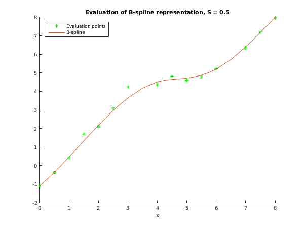
Calling with smoothing factor S = 0.50
Knots Coeffs
1 -1.1072
2 0.0000 -0.6571
3 1.0000 0.4350
4 2.0000 2.8061
5 4.0000 4.6824
6 5.0000 4.6416
7 6.0000 5.1976
8 8.0000 6.9008
9 7.9979
Weighted sum of squared residuals = 0.5001
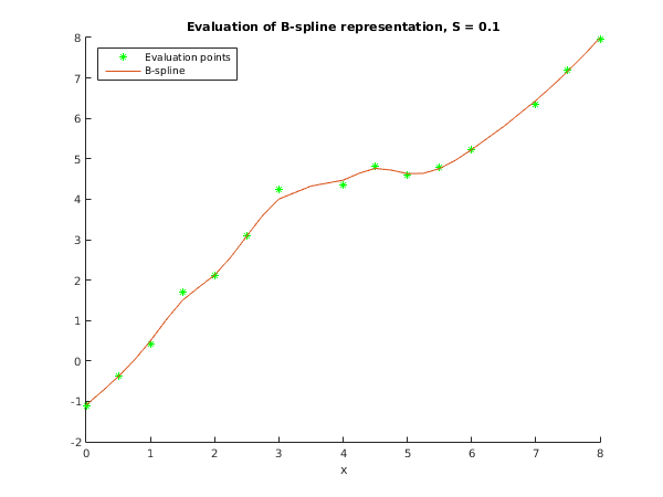
Calling with smoothing factor S = 0.10
Knots Coeffs
1 -1.0901
2 0.0000 -0.6401
3 1.0000 0.0334
4 1.5000 1.6390
5 2.0000 2.1243
6 3.0000 4.5591
7 4.0000 4.2174
8 4.5000 4.9105
9 5.0000 4.5475
10 5.5000 4.6960
11 6.0000 5.7370
12 8.0000 6.8179
13 7.9953
Weighted sum of squared residuals = 0.1000
PDF version (NAG web site
, 64-bit version, 64-bit version)
© The Numerical Algorithms Group Ltd, Oxford, UK. 2009–2015