PDF version (NAG web site
, 64-bit version, 64-bit version)
NAG Toolbox: nag_correg_lars_xtx (g02mb)
Purpose
nag_correg_lars_xtx (g02mb) performs Least Angle Regression (LARS), forward stagewise linear regression or Least Absolute Shrinkage and Selection Operator (LASSO) using cross-product matrices.
Syntax
[
b,
fitsum,
ifail] = g02mb(
mtype,
n,
dtd,
dty,
yty, 'pred',
pred, 'intcpt',
intcpt, 'm',
m, 'isx',
isx, 'mnstep',
mnstep, 'ropt',
ropt)
[
b,
fitsum,
ifail] = nag_correg_lars_xtx(
mtype,
n,
dtd,
dty,
yty, 'pred',
pred, 'intcpt',
intcpt, 'm',
m, 'isx',
isx, 'mnstep',
mnstep, 'ropt',
ropt)
Description
nag_correg_lars_xtx (g02mb) implements the LARS algorithm of
Efron et al. (2004) as well as the modifications needed to perform forward stagewise linear regression and fit LASSO and positive LASSO models.
Given a vector of
observed values,
and an
design matrix
, where the
th column of
, denoted
, is a vector of length
representing the
th independent variable
, standardized such that
, and
and a set of model parameters
to be estimated from the observed values, the LARS algorithm can be summarised as:
| 1. |
Set and all coefficients to zero, that is . |
| 2. |
Find the variable most correlated with , say . Add to the ‘most correlated’ set . If go to 8. |
| 3. |
Take the largest possible step in the direction of (i.e., increase the magnitude of ) until some other variable, say , has the same correlation with the current residual, . |
| 4. |
Increment and add to . |
| 5. |
If go to 8. |
| 6. |
Proceed in the ‘least angle direction’, that is, the direction which is equiangular between all variables in , altering the magnitude of the parameter estimates of those variables in , until the th variable, , has the same correlation with the current residual. |
| 7. |
Go to 4. |
| 8. |
Let . |
As well as being a model selection process in its own right, with a small number of modifications the LARS algorithm can be used to fit the LASSO model of
Tibshirani (1996), a positive LASSO model, where the independent variables enter the model in their defined direction, forward stagewise linear regression (
Hastie et al. (2001)) and forward selection (
Weisberg (1985)). Details of the required modifications in each of these cases are given in
Efron et al. (2004).
The LASSO model of
Tibshirani (1996) is given by
for all values of
, where
. The positive LASSO model is the same as the standard LASSO model, given above, with the added constraint that
Unlike the standard LARS algorithm, when fitting either of the LASSO models, variables can be dropped as well as added to the set . Therefore the total number of steps is no longer bounded by .
Forward stagewise linear regression is an iterative procedure of the form:
| 1. |
Initialize and the vector of residuals . |
| 2. |
For each calculate . The value is therefore proportional to the correlation between the th independent variable and the vector of previous residual values, . |
| 3. |
Calculate , the value of with the largest absolute value of . |
| 4. |
If then go to 7. |
| 5. |
Update the residual values, with
where is a small constant and when and otherwise. |
| 6. |
Increment and go to 2. |
| 7. |
Set . |
If the largest possible step were to be taken, that is
then forward stagewise linear regression reverts to the standard forward selection method as implemented in
nag_correg_linregm_fit_onestep (g02ee).
The LARS procedure results in
models, one for each step of the fitting process. In order to aid in choosing which is the most suitable
Efron et al. (2004) introduced a
-type statistic given by
where
is the approximate degrees of freedom for the
th step and
One way of choosing a model is therefore to take the one with the smallest value of .
References
Efron B, Hastie T, Johnstone I and Tibshirani R (2004) Least Angle Regression The Annals of Statistics (Volume 32) 2 407–499
Hastie T, Tibshirani R and Friedman J (2001) The Elements of Statistical Learning: Data Mining, Inference and Prediction Springer (New York)
Tibshirani R (1996) Regression Shrinkage and Selection via the Lasso Journal of the Royal Statistics Society, Series B (Methodological) (Volume 58) 1 267–288
Weisberg S (1985) Applied Linear Regression Wiley
Parameters
Compulsory Input Parameters
- 1:
– int64int32nag_int scalar
-
Indicates the type of model to fit.
- LARS is performed.
- Forward linear stagewise regression is performed.
- LASSO model is fit.
- A positive LASSO model is fit.
Constraint:
, , or .
- 2:
– int64int32nag_int scalar
-
, the number of observations.
Constraint:
.
- 3:
– double array
-
The the array
dtd must be a vector of length at least
or a matrix of size at least (
,
)
, the cross-product matrix, which along with
isx, defines the design matrix cross-product
.
If supplied in compressed format,
must contain the cross-product of the
th and
th variable, for
and
. That is the cross-product stacked by columns as returned by
nag_correg_ssqmat (g02bu), for example.
Otherwise
must contain the cross-product of the th and th variable, for and . It should be noted that, even though is symmetric, the full matrix must be supplied.
The matrix specified in
dtd must be a valid cross-products matrix.
- 4:
– double array
-
, the cross-product between the dependent variable, , and the independent variables .
- 5:
– double scalar
-
, the sums of squares of the dependent variable.
Constraint:
.
Optional Input Parameters
- 1:
– int64int32nag_int scalar
Default:
Indicates the type of preprocessing to perform on the cross-products involving the independent variables, i.e., those supplied in
dtd and
dty.
- No preprocessing is performed.
- Each independent variable is normalized, with the th variable scaled by . The scaling factor used by variable is returned in .
Constraint:
or .
- 2:
– int64int32nag_int scalar
Default:
Indicates the type of data preprocessing that was perform on the dependent variable,
, prior to calling this function.
- No preprocessing was performed.
- The dependent variable, , was mean centered.
Constraint:
or .
- 3:
– int64int32nag_int scalar
-
Default:
the second dimension of the array
dtd and the dimension of the array
dty. (An error is raised if these dimensions are not equal.)
, the total number of independent variables when all variables are included.
Constraint:
.
- 4:
– int64int32nag_int array
-
Indicates which independent variables from
dtd will be included in the design matrix,
.
If
isx is not supplied, all variables are included in the design matrix.
Otherwise,, for
when
must be set as follows:
- To indicate that the th variable, as supplied in dtd, is included in the design matrix;
- To indicate that the th variable, as supplied in dtd, is not included in the design matrix;
and
Constraint:
or and at least one value of , for .
- 5:
– int64int32nag_int scalar
Default:
- if , ;
- otherwise .
The maximum number of steps to carry out in the model fitting process.
If , i.e., a LARS is being performed, the maximum number of steps the algorithm will take is if , otherwise .
If , i.e., a forward linear stagewise regression is being performed, the maximum number of steps the algorithm will take is likely to be several orders of magnitude more and is no longer bound by or .
If or , i.e., a LASSO or positive LASSO model is being fit, the maximum number of steps the algorithm will take lies somewhere between that of the LARS and forward linear stagewise regression, again it is no longer bound by or .
Constraint:
.
- 6:
– double array
-
Optional parameters to control various aspects of the LARS algorithm.
The default value will be used for
if
. The default value will also be used if an invalid value is supplied for a particular argument, for example, setting
will use the default value for argument
.
- The minimum step size that will be taken.
Default is
is used, where
is the
machine precision returned by
nag_machine_precision (x02aj).
- General tolerance, used amongst other things, for comparing correlations.
Default is .
- If set to then parameter estimates are rescaled before being returned. If set to then no rescaling is performed. This argument has no effect when .
Default is for the parameter estimates to be rescaled.
Constraints:
- ;
- .
Output Parameters
- 1:
– double array
-
The second dimension of the array
b will be
.
Note: nstep is equal to
, the actual number of steps carried out in the model fitting process. See
Description for further information.
the parameter estimates, with
, the parameter estimate for the
th variable,
at the
th step of the model fitting process,
.
The number of parameter estimates,
, is the number of variables in
dtd when
isx is not supplied, i.e.,
. Otherwise
is the number of nonzero values in
isx.
By default, when
the parameter estimates are rescaled prior to being returned. If the parameter estimates are required on the normalized scale, then this can be overridden via
ropt.
The values held in the remaining part of
b depend on the type of preprocessing performed.
for .
- 2:
– double array
-
The second dimension of the array
fitsum will be
.
Summaries of the model fitting process. When
- , the sum of the absolute values of the parameter estimates for the th step of the modelling fitting process. If , the scaled parameter estimates are used in the summation.
- , the residual sums of squares for the th step, where .
- , approximate degrees of freedom for the th step.
- , a -type statistic for the th step, where .
- , correlation between the residual at step and the most correlated variable not yet in the active set , where the residual at step is .
- , the step size used at step .
In addition
- .
- , the residual sums of squares for the null model, where .
- , the degrees of freedom for the null model, where if and otherwise.
- , a -type statistic for the null model, where .
- , where and .
Although the statistics described above are returned when they may not be meaningful due to the estimate not being based on the saturated model.
- 3:
– int64int32nag_int scalar
unless the function detects an error (see
Error Indicators and Warnings).
Error Indicators and Warnings
Note: nag_correg_lars_xtx (g02mb) may return useful information for one or more of the following detected errors or warnings.
Errors or warnings detected by the function:
Cases prefixed with W are classified as warnings and
do not generate an error of type NAG:error_n. See nag_issue_warnings.
-
-
Constraint: , , or .
-
-
Constraint: or .
-
-
Constraint: or .
-
-
Constraint: .
-
-
Constraint: .
-
-
The cross-product matrix supplied in
dtd is not symmetric.
-
-
Constraint: diagonal elements of must be positive.
-
-
Constraint: or for all .
-
-
On entry, all values of
isx are zero.
Constraint: at least one value of
isx must be nonzero.
-
-
Constraint: .
-
-
A negative value for the residual sums of squares was obtained. Check the values of
dtd,
dty and
yty.
-
-
Constraint: .
- W
-
Fitting process did not finished in
mnstep steps. Try increasing the size of
mnstep.
All output is returned as documented, up to step
mnstep, however,
and the
statistics may not be meaningful.
- W
-
is approximately zero and hence the -type criterion cannot be calculated. All other output is returned as documented.
- W
-
, therefore sigma has been set to a large value. Output is returned as documented.
- W
-
Degenerate model, no variables added and . Output is returned as documented.
-
-
Constraint: .
-
An unexpected error has been triggered by this routine. Please
contact
NAG.
-
Your licence key may have expired or may not have been installed correctly.
-
Dynamic memory allocation failed.
Accuracy
Not applicable.
Further Comments
The solution path to the LARS, LASSO and stagewise regression analysis is a continuous, piecewise linear.
nag_correg_lars_xtx (g02mb) returns the parameter estimates at various points along this path.
nag_correg_lars_param (g02mc) can be used to obtain estimates at different points along the path.
If you have the raw data values, that is
and
, then
nag_correg_lars (g02ma) can be used instead of
nag_correg_lars_xtx (g02mb).
Example
This example performs a LARS on a simulated dataset with observations and independent variables.
The example uses
nag_correg_ssqmat (g02bu) to get the cross-products of the augmented matrix
. The first
elements of the (column packed) cross-products matrix returned therefore contain the elements of
, the next
elements contain
and the last element
.
Open in the MATLAB editor:
g02mb_example
function g02mb_example
fprintf('g02mb example results\n\n');
mtype = int64(1);
dy = [10.28 1.77 9.69 15.58 8.23 10.44 -46.47;
9.08 8.99 11.53 6.57 15.89 12.58 -35.80;
17.98 13.10 1.04 10.45 10.12 16.68 -129.22;
14.82 13.79 12.23 7.00 8.14 7.79 -42.44;
17.53 9.41 6.24 3.75 13.12 17.08 -73.51;
7.78 10.38 9.83 2.58 10.13 4.25 -26.61;
11.95 21.71 8.83 11.00 12.59 10.52 -63.90;
14.60 10.09 -2.70 9.89 14.67 6.49 -76.73;
3.63 9.07 12.59 14.09 9.06 8.19 -32.64;
6.35 9.79 9.40 12.79 8.38 16.79 -83.29;
4.66 3.55 16.82 13.83 21.39 13.88 -16.31;
8.32 14.04 17.17 7.93 7.39 -1.09 -5.82;
10.86 13.68 5.75 10.44 10.36 10.06 -47.75;
4.76 4.92 17.83 2.90 7.58 11.97 18.38;
5.05 10.41 9.89 9.04 7.90 13.12 -54.71;
5.41 9.32 5.27 15.53 5.06 19.84 -55.62;
9.77 2.37 9.54 20.23 9.33 8.82 -45.28;
14.28 4.34 14.23 14.95 18.16 11.03 -22.76;
10.17 6.80 3.17 8.57 16.07 15.93 -104.32;
5.39 2.67 6.37 13.56 10.68 7.35 -55.94];
n = int64(size(dy,1));
mean_p = 'M';
[~,wmean,dtd,ifail] = g02bu( ...
dy,'mean_p',mean_p);
m = int64(size(dy,2) - 1);
pm = m*(m+1)/2;
warn_state = nag_issue_warnings();
nag_issue_warnings(true);
[b,fitsum,ifail] = g02mb( ...
mtype,n,dtd(1:pm),dtd((pm+1):(pm+m)),dtd(end));
nag_issue_warnings(warn_state);
ip = size(b,1);
nstep = size(b,2) - 1;
fprintf(' Step %s Parameter Estimate\n ',repmat(' ',1,max(ip-2,0)*5));
fprintf(repmat('-',1,5+ip*10));
fprintf('\n');
for k = 1:nstep
fprintf(' %3d',k);
for j = 1:ip
fprintf(' %9.3f',b(j,k));
end
fprintf('\n');
end
fprintf('\n');
fprintf(' alpha: %9.3f\n', wmean(m+1));
fprintf('\n');
fprintf(' Step Sum RSS df Cp Ck Step Size\n ');
fprintf(repmat('-',1,64));
fprintf('\n');
for k = 1:nstep
fprintf(' %3d %9.3f %9.3f %6.0f %9.3f %9.3f %9.3f\n', ...
k,fitsum(1,k),fitsum(2,k),fitsum(3,k), ...
fitsum(4,k),fitsum(5,k),fitsum(6,k));
end
fprintf('\n');
fprintf(' sigma^2: %9.3f\n', fitsum(5,nstep+1));
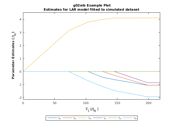
fig1 = figure;
ip = size(b,1);
nstep = size(b,2) - 2;
xpos = transpose(repmat(fitsum(1,1:nstep),ip,1));
ypos = transpose(b(1:ip,1:nstep));
xpos = [zeros(1,ip);xpos];
ypos = [zeros(1,ip);ypos];
xmin = min(min(xpos));
xmax = max(max(xpos));
ymin = min(min(ypos));
ymax = max(max(ypos));
ext = 1 + [-0.1 0.1];
xrng = [min(xmin*ext),max(xmax*ext)];
yrng = [min(ymin*ext),max(ymax*ext)];
xpos = [xpos;xrng(2)*ones(1,ip)];
ypos = [ypos;ypos(end,:)];
plot(xpos,ypos);
xlim(xrng);
ylim(yrng);
title({'{\bf g02mb Example Plot}'; ...
'Estimates for LAR model fitted to simulated dataset'});
xlabel('{\bf \Sigma_j |\beta_{kj} |}');
ylabel('{\bf Parameter Estimates (\beta_{kj})}');
label = [repmat('\beta_{k',ip,1) num2str(transpose(linspace(1,ip,ip))) ...
repmat('}',ip,1)];
h = legend(label,'Location','SouthOutside','Orientation','Horizontal');
set(h,'FontSize',get(h,'FontSize')*0.8);
g02mb example results

  Step                      Parameter Estimate
 -----------------------------------------------------------------
    1     0.000     0.000     3.125     0.000     0.000     0.000
    2     0.000     0.000     3.792     0.000     0.000    -0.713
    3    -0.446     0.000     3.998     0.000     0.000    -1.151
    4    -0.628    -0.295     4.098     0.000     0.000    -1.466
    5    -1.060    -1.056     4.110    -0.864     0.000    -1.948
    6    -1.073    -1.132     4.118    -0.935    -0.059    -1.981

 alpha:   -50.037

  Step     Sum      RSS       df       Cp       Ck     Step Size
 ----------------------------------------------------------------
    1    72.446  8929.855      2     13.355   123.227    72.446
    2   103.385  6404.701      3      7.054    50.781    24.841
    3   126.243  5258.247      4      5.286    30.836    16.225
    4   145.277  4657.051      5      5.309    19.319    11.587
    5   198.223  3959.401      6      5.016    12.266    24.520
    6   203.529  3954.571      7      7.000     0.910     2.198

 sigma^2:   304.198
This example plot shows the regression coefficients () plotted against the scaled absolute sum of the parameter estimates ().
PDF version (NAG web site
, 64-bit version, 64-bit version)
© The Numerical Algorithms Group Ltd, Oxford, UK. 2009–2015