d02pw:: Ordinary Differential EquationsIntegrators for Stiff Ordinary Differential Systems (NAG Toolbox)

This example integrates a two body problem. The equations for the coordinates

(x (t), y (t))

of one body as functions of time

t

in a suitable frame of reference are

x^{''} = - \frac{x}{r^{3}}

y^{''} = - \frac{y}{r^{3}}, r = \sqrt{x^{2} + y^{2}} .

The initial conditions

\begin{array}{l} x (0) = 1 - ε, & x^{'} (0) = 0 \\ y (0) = 0, & y^{'} (0) = \sqrt{\frac{1 + ε}{1 - ε}} \end{array}

lead to elliptic motion with

0 < ε < 1

ε = 0.7

is selected and reposed as

\begin{array}{l} y_{1}^{'} = y_{3} \\ y_{2}^{'} = y_{4} \\ y_{3}^{'} = - \frac{y_{1}}{r^{3}} \\ y_{4}^{'} = - \frac{y_{2}}{r^{3}} \end{array}

over the range

[0, 6 π]

. Relative error control is used with threshold values of

1.0e−10

for each solution component and compute the solution at intervals of length

π

across the range using nag_ode_ivp_rk_reset_tend (d02pw) to reset the end of the integration range. A high-order Runge–Kutta method (

method = 3

) is also used with tolerances

tol = 1.0e−4

and

tol = 1.0e−5

in turn so that the solutions may be compared. The value of

π

is obtained by using nag_math_pi (x01aa).

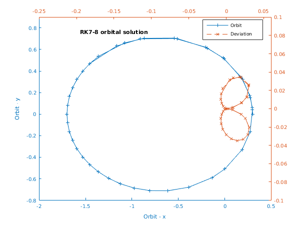
function d02pw_example


fprintf('d02pw example results\n\n');

% Initialize variables and arrays.
neq = int64(4);
lenwrk = int64(32*neq);
method = int64(3);
ecc = 0.7;

tstart = 0.0;
ystart = [1.0-ecc; 0.0; 0.0; sqrt((1.0+ecc)/(1.0-ecc))];
tend = 6.0*pi;
thres = [1e-10; 1e-10; 1e-10; 1e-10];
task = 'Complex Task';  % tell d02pv to use d02pd.
errass = false;
hstart = 0.0;

% We run through the calculation twice: once to output the results at
% a collection of points, and again to accumulate a series of results for
% plotting.
nstep = [6; 96];

% Prepare to accumulate results.  The first and last points should be the
% same - i.e. so the plot shows a closed trajectory.
xarray = zeros(nstep(2)+1, 1);
yarray = zeros(nstep(2)+1, 4);

for icalc = 1:2
  tinc  = tend/nstep(icalc);

  % For each calculation, use two tolerances;
  % plot results corresponding to the second one.
  tol = [1.0e-4; 1.0e-5];
  for itol = 1:2;

    istep = 1;
    twant = tinc;

    % d02pv is a setup routine to be called prior to d02pd.
    [work, ifail] = d02pv( ...
                           tstart, ystart, twant, tol(itol), thres, method, ...
                           task, errass, lenwrk, 'neq', neq, 'hstart', hstart);

    if icalc == 1
      % Output initial results.
      fprintf('Calculation with tol = %1.1e\n\n',tol(itol));
      fprintf('   t         y1        y2        y3        y4\n');
      fprintf(' %6.3f', tstart);
      for ieq = 1:neq
        fprintf('  %8.4f', ystart(ieq));
      end
      fprintf('\n');
    else
      % Store current results.
      xarray(1) = tstart;
      for ieq = 1:neq
        yarray(1, ieq) = ystart(ieq);
      end
    end

    tnow = 0.0;
    while tnow < tend
      if icalc == 1
        % For the first calculation, keep integrating till the
        % (current value for the) endpoint is reached.
        while tnow < twant
          [tnow, ynow, ypnow, work, ifail] = ...
          d02pd( ...
                 @f, neq, work);
        end
        % Output current result.
        fprintf(' %6.3f', tnow);
        for ieq = 1:neq
          fprintf('  %8.4f', ynow(ieq));
        end
        fprintf('\n');
      else
        % For the second calculation, just take a single step.
        [tnow, ynow, ypnow, work, ifail] = ...
        d02pd( ...
               @f, neq, work);
        % Store current result.
        xarray(istep+1) = tnow;
        for ieq = 1:neq
          yarray(istep+1, ieq) = ynow(ieq);
        end
      end

      % Update the endpoint, and call d02pw to reset it.
      istep = istep + 1;
      twant = istep*tinc;
      [ifail] = d02pw(twant);
    end

    if icalc == 1
      % d02py is a diagnostic routine.
      [totfcn, stpcst, waste, stpsok, hnext, ifail] = ...
      d02py;
      fprintf(['\nCost of the integration in evaluations of ', ...
               'F is %1.0f\n\n\n'], totfcn);
    end
  end
end

% Use the first two components of the solution, and calculate the deviation
% from a true ellipse.
x = yarray(:,1);
y = yarray(:,2);
xdev = zeros(nstep(2)+1, 1);
ydev = zeros(nstep(2)+1, 1);
for i = 1:nstep(2)+1
  fac = abs((x(i) + ecc)*(x(i) + ecc) + y(i)*y(i)/(ecc*ecc) - 1.0);
  xdev(i) = fac*cos(xarray(i));
  ydev(i) = fac*sin(xarray(i));
end
% Plot results.
fig1 = figure;
display_plot(x, y, xdev, ydev);


function [yp] = f(t, y, yp)
  % Evaluate derivative vector.

  yp = zeros(4, 1);
  r = sqrt((y(1)^2 + y(2)^2));
  yp(1) =  y(3);
  yp(2) =  y(4);
  yp(3) = -y(1)/r^3;
  yp(4) = -y(2)/r^3;

function display_plot(x1, y1, x2, y2)
  % Plot the results.  First, get the list of default colours (we have to
  % specify the plot colours by hand).
  axes('XLim', [-2 0.5], 'YLim', [-0.8 0.9]);
  cols = get(gca, 'ColorOrder');
  % Plot the first curve.
  hline1 = line(x1, y1, 'Color', cols(1,:));
  ax1 = gca;
  set(ax1, 'XColor', cols(1,:), 'YColor', cols(1,:));
  % Label these axes.
  xlabel('Orbit - x');
  ylabel('Orbit - y');
  % Set up the second set of axes and plot the second curve.
  ax2 = axes('Position', get(ax1,'Position'), ...
             'XAxisLocation', 'top', 'YAxisLocation', 'right', ...
             'Color','none', 'XColor',cols(2,:), 'YColor', cols(2,:), ...
             'XLim', [-0.25 0.06], 'YLim', [-0.1 0.1]);
  hline2 = line(x2, y2, 'Color', cols(2,:), 'Parent', ax2);
  % Label these axes.
  h = title('RK7-8 orbital solution');
  set(h,'Position',[-0.15,0.08]);
  % Add a legend, specifying the lines explicitly.
  legend([hline1, hline2],'Orbit','Deviation','Location','Best');
  % Set some features of the two lines.
  set(hline1, 'Linewidth', 0.25, 'Marker', '+', 'LineStyle', '-');
  set(hline2, 'Linewidth', 0.25, 'Marker', 'x', 'LineStyle', '--');

NAG Toolbox: nag_ode_withdraw_ivp_rk_reset_tend (d02pw)

▸▿ Contents

Purpose

Syntax

Description

References

Parameters

Compulsory Input Parameters

Optional Input Parameters

Output Parameters

Error Indicators and Warnings

Accuracy

Further Comments

Example

References

Brankin R W, Gladwell I and Shampine L F (1991) RKSUITE: A suite of Runge–Kutta codes for the initial value problems for ODEs SoftReport 91-S1 Southern Methodist University