PDF version (NAG web site
, 64-bit version, 64-bit version)
NAG Toolbox: nag_ode_bvp_coll_nlin_setup (d02tv)
Purpose
nag_ode_bvp_coll_nlin_setup (d02tv) is a setup function which must be called prior to the first call of the nonlinear two-point boundary value solver
nag_ode_bvp_coll_nlin_solve (d02tl).
Syntax
[
rcomm,
icomm,
ifail] = d02tv(
m,
nlbc,
nrbc,
ncol,
tols,
nmesh,
mesh,
ipmesh, 'neq',
neq, 'mxmesh',
mxmesh, 'lrcomm',
lrcomm, 'licomm',
licomm)
[
rcomm,
icomm,
ifail] = nag_ode_bvp_coll_nlin_setup(
m,
nlbc,
nrbc,
ncol,
tols,
nmesh,
mesh,
ipmesh, 'neq',
neq, 'mxmesh',
mxmesh, 'lrcomm',
lrcomm, 'licomm',
licomm)
Description
nag_ode_bvp_coll_nlin_setup (d02tv) and its associated functions (
nag_ode_bvp_coll_nlin_solve (d02tl),
nag_ode_bvp_coll_nlin_contin (d02tx),
nag_ode_bvp_coll_nlin_interp (d02ty) and
nag_ode_bvp_coll_nlin_diag (d02tz)) solve the two-point boundary value problem for a nonlinear system of ordinary differential equations
over an interval
subject to
(
) nonlinear boundary conditions at
and
(
) nonlinear boundary conditions at
, where
. Note that
is the
th derivative of the
th solution component. Hence
. The left boundary conditions at
are defined as
and the right boundary conditions at
as
where
and
See
Further Comments for information on how boundary value problems of a more general nature can be treated.
nag_ode_bvp_coll_nlin_setup (d02tv) is used to specify an initial mesh, error requirements and other details.
nag_ode_bvp_coll_nlin_solve (d02tl) is then used to solve the boundary value problem.
The solution function
nag_ode_bvp_coll_nlin_solve (d02tl) proceeds as follows. A modified Newton method is applied to the equations
and the boundary conditions. To solve these equations numerically the components
are approximated by piecewise polynomials
using a monomial basis on the
th mesh sub-interval. The coefficients of the polynomials
form the unknowns to be computed. Collocation is applied at Gaussian points
where
is the
th collocation point in the
th mesh sub-interval. Continuity at the mesh points is imposed, that is
where
is the right-hand end of the
th mesh sub-interval. The linearized collocation equations and boundary conditions, together with the continuity conditions, form a system of linear algebraic equations, an almost block diagonal system which is solved using special linear solvers. To start the modified Newton process, an approximation to the solution on the initial mesh must be supplied via the procedure argument
guess of
nag_ode_bvp_coll_nlin_solve (d02tl).
The solver attempts to satisfy the conditions
where
is the approximate solution for the
th solution component and
tols is supplied by you. The mesh is refined by trying to equidistribute the estimated error in the computed solution over all mesh sub-intervals, and an extrapolation-like test (doubling the number of mesh sub-intervals) is used to check for
(1).
The functions are based on modified versions of the codes COLSYS and COLNEW (see
Ascher et al. (1979) and
Ascher and Bader (1987)). A comprehensive treatment of the numerical solution of boundary value problems can be found in
Ascher et al. (1988) and
Keller (1992).
References
Ascher U M and Bader G (1987) A new basis implementation for a mixed order boundary value ODE solver SIAM J. Sci. Stat. Comput. 8 483–500
Ascher U M, Christiansen J and Russell R D (1979) A collocation solver for mixed order systems of boundary value problems Math. Comput. 33 659–679
Ascher U M, Mattheij R M M and Russell R D (1988) Numerical Solution of Boundary Value Problems for Ordinary Differential Equations Prentice–Hall
Gill P E, Murray W and Wright M H (1981) Practical Optimization Academic Press
Keller H B (1992) Numerical Methods for Two-point Boundary-value Problems Dover, New York
Schwartz I B (1983) Estimating regions of existence of unstable periodic orbits using computer-based techniques SIAM J. Sci. Statist. Comput. 20(1) 106–120
Parameters
Compulsory Input Parameters
- 1:
– int64int32nag_int array
-
must contain , the order of the th differential equation, for .
Constraint:
, for .
- 2:
– int64int32nag_int scalar
-
, the number of left boundary conditions defined at the left-hand end, ().
Constraint:
.
- 3:
– int64int32nag_int scalar
-
, the number of right boundary conditions defined at the right-hand end, ().
Constraints:
- ;
- .
- 4:
– int64int32nag_int scalar
-
The number of collocation points to be used in each mesh sub-interval.
Constraint:
, where .
- 5:
– double array
-
must contain the error requirement for the th solution component.
Constraint:
, for .
- 6:
– int64int32nag_int scalar
-
The number of points to be used in the initial mesh of the solution process.
Constraint:
.
- 7:
– double array
-
The positions of the initial
nmesh mesh points. The remaining elements of
mesh need not be set. You should try to place the mesh points in areas where you expect the solution to vary most rapidly. In the absence of any other information the points should be equally distributed on
.
must contain the left boundary point, , and must contain the right boundary point, .
Constraint:
, for .
- 8:
– int64int32nag_int array
-
specifies whether or not the initial mesh point defined in
, for
, should be a fixed point in all meshes computed during the solution process. The remaining elements of
ipmesh need not be set.
- Indicates that should be a fixed point in all meshes.
- Indicates that is not a fixed point.
Constraints:
- and , (i.e., the left and right boundary points, and , must be fixed points, in all meshes);
- or , for .
Optional Input Parameters
- 1:
– int64int32nag_int scalar
-
Default:
the dimension of the arrays
m,
tols. (An error is raised if these dimensions are not equal.)
, the number of ordinary differential equations to be solved.
Constraint:
.
- 2:
– int64int32nag_int scalar
-
Default:
the dimension of the arrays
mesh,
ipmesh. (An error is raised if these dimensions are not equal.)
The maximum number of mesh points to be used during the solution process.
Constraint:
.
- 3:
– int64int32nag_int scalar
Suggested value:
, which will permit
mxmesh mesh points for a system of
neq differential equations regardless of their order or the number of collocation points used.
Default:
The dimension of the array
rcomm. if
, a communication array size query is requested. In this case there is an immediate return with communication array dimensions stored in
icomm;
contains the required dimension of
rcomm, while
contains the required dimension of
icomm.
Constraint:
, or , where and .
- 4:
– int64int32nag_int scalar
Suggested value:
, which will permit
mxmesh mesh points for a system of
neq differential equations regardless of their order or the number of collocation points used.
Default:
The dimension of the array
icomm. if
, a communication array size query is requested. In this case
icomm need only be of dimension
in order to hold the required communication array dimensions for the given problem and algorithmic parameters.
Constraints:
- if , ;
- otherwise .
Output Parameters
- 1:
– double array
-
Contains information for use by
nag_ode_bvp_coll_nlin_solve (d02tl). This
must be the same array as will be supplied to
nag_ode_bvp_coll_nlin_solve (d02tl). The contents of this array
must remain unchanged between calls.
- 2:
– int64int32nag_int array
-
Contains information for use by
nag_ode_bvp_coll_nlin_solve (d02tl). This
must be the same array as will be supplied to
nag_ode_bvp_coll_nlin_solve (d02tl). The contents of this array
must remain unchanged between calls. If
, a communication array size query is requested. In this case, on immediate return,
will contain the required dimension for
rcomm while
will contain the required dimension for
icomm.
- 3:
– int64int32nag_int scalar
unless the function detects an error (see
Error Indicators and Warnings).
Error Indicators and Warnings
Errors or warnings detected by the function:
-
-
Constraint: for all .
Constraint: or .
Constraint: .
Constraint: .
Constraint: .
Constraint: .
Constraint: and .
Constraint: .
Constraint: for all .
On entry, or does not equal .
On entry, or for some .
On entry, the elements of
mesh are not strictly increasing.
-
An unexpected error has been triggered by this routine. Please
contact
NAG.
-
Your licence key may have expired or may not have been installed correctly.
-
Dynamic memory allocation failed.
Accuracy
Not applicable.
Further Comments
For problems where sharp changes of behaviour are expected over short intervals it may be advisable to:
| – |
use a large value for ncol; |
| – |
cluster the initial mesh points where sharp changes in behaviour are expected; |
| – |
maintain fixed points in the mesh using the argument ipmesh to ensure that the remeshing process does not inadvertently remove mesh points from areas of known interest before they are detected automatically by the algorithm. |
Nonseparated Boundary Conditions
A boundary value problem with nonseparated boundary conditions can be treated by transformation to an equivalent problem with separated conditions. As a simple example consider the system
on
subject to the boundary conditions
By adjoining the trivial ordinary differential equation
which implies
, and letting
, say, we have a new system
subject to the separated boundary conditions
There is an obvious overhead in adjoining an extra differential equation: the system to be solved is increased in size.
Multipoint Boundary Value Problems
Multipoint boundary value problems, that is problems where conditions are specified at more than two points, can also be transformed to an equivalent problem with two boundary points. Each sub-interval defined by the multipoint conditions can be transformed onto the interval
, say, leading to a larger set of differential equations. The boundary conditions of the transformed system consist of the original boundary conditions and the conditions imposed by the requirement that the solution components be continuous at the interior break-points. For example, consider the equation
subject to the conditions
where
. This can be transformed to the system
where
subject to the boundary conditions
In this instance two of the resulting boundary conditions are nonseparated but they may next be treated as described above.
High Order Systems
Systems of ordinary differential equations containing derivatives of order greater than four can always be reduced to systems of order suitable for treatment by
nag_ode_bvp_coll_nlin_setup (d02tv) and its related functions. For example suppose we have the sixth-order equation
Writing the variables
and
we obtain the system
which has maximal order four, or writing the variables
and
we obtain the system
which has maximal order three. The best choice of reduction by choosing new variables will depend on the structure and physical meaning of the system. Note that you will control the error in each of the variables
and
. Indeed, if you wish to control the error in certain derivatives of the solution of an equation of order greater than one, then you should make those derivatives new variables.
Fixed Points and Singularities
The solver function
nag_ode_bvp_coll_nlin_solve (d02tl) employs collocation at Gaussian points in each sub-interval of the mesh. Hence the coefficients of the differential equations are not evaluated at the mesh points. Thus, fixed points should be specified in the mesh where either the coefficients are singular, or the solution has less smoothness, or where the differential equations should not be evaluated. Singular coefficients at boundary points often arise when physical symmetry is used to reduce partial differential equations to ordinary differential equations. These do not pose a direct numerical problem for using this code but they can severely impact its convergence.
Numerical Jacobians
The solver function
nag_ode_bvp_coll_nlin_solve (d02tl) requires an external function
fjac to evaluate the partial derivatives of
with respect to the elements of
(
). In cases where the partial derivatives are difficult to evaluate, numerical approximations can be used. However, this approach might have a negative impact on the convergence of the modified Newton method. You could consider the use of symbolic mathematic packages and/or automatic differentiation packages if available to you.
See
Example in
nag_ode_bvp_coll_nlin_diag (d02tz) for an example using numerical approximations to the Jacobian. There central differences are used and each
is assumed to depend on all the components of
. This requires two evaluations of the system of differential equations for each component of
. The perturbation used depends on the size of each component of
and a minimum quantity dependent on the
machine precision. The cost of this approach could be reduced by employing an alternative difference scheme and/or by only perturbing the components of
which appear in the definitions of the
. A discussion on the choice of perturbation factors for use in finite difference approximations to partial derivatives can be found in
Gill et al. (1981).
Example
The following example is used to illustrate the treatment of nonseparated boundary conditions. See also
nag_ode_bvp_coll_nlin_solve (d02tl),
nag_ode_bvp_coll_nlin_contin (d02tx),
nag_ode_bvp_coll_nlin_interp (d02ty) and
nag_ode_bvp_coll_nlin_diag (d02tz), for the illustration of other facilities.
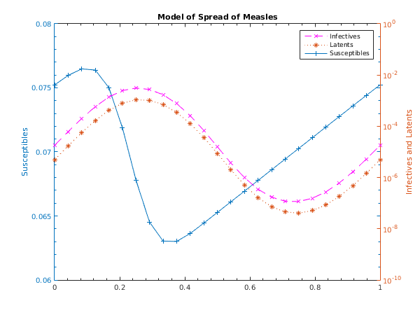
The following equations model of the spread of measles. See
Schwartz (1983). Under certain assumptions the dynamics of the model can be expressed as
subject to the periodic boundary conditions
Here
and
are respectively the proportions of susceptibles, infectives and latents to the whole population.
(
years) is the latent period,
(
years) is the infectious period and
(
) is the population birth rate.
is the contact rate where
.
The nonseparated boundary conditions are treated as described in
Further Comments by adjoining the trivial differential equations
that is
and
are constants. The boundary conditions of the augmented system can then be posed in the separated form
This is a relatively easy problem and an (arbitrary) initial guess of
for each component suffices, even though two components of the solution are much smaller than
.
Open in the MATLAB editor:
d02tv_example
function d02tv_example
fprintf('d02tv example results\n\n');
global beta0 eta lambda mu
eta = 0.01;
mu = 0.02;
lambda = 0.0279;
beta0 = 1575.0;
neq = int64(6);
nlbc = int64(3);
nrbc = nlbc;
ncol = int64(5);
mmax = int64(1);
nmesh = int64(7);
mxmesh = int64(8*nmesh);
ipmesh = zeros(mxmesh, 1, 'int64');
mesh = zeros(mxmesh, 1);
mstep = 1/double(nmesh-1);
mesh(1:nmesh) = 0:mstep:1;
ipmesh(1:nmesh) = int64(2);
ipmesh(1) = int64(1);
ipmesh(nmesh) = int64(1);
m(1:neq) = int64(1);
tols(1:neq) = 1e-6;
[work, iwork, ifail] = d02tv(...
m, nlbc, nrbc, ncol, tols, nmesh, mesh, ipmesh);
[work, iwork, ifail] = d02tk(...
@ffun, @fjac, @gafun, @gbfun, @gajac, @gbjac,...
@guess, work, iwork);
[nmesh, mesh, ipmesh, ermx, iermx, ijermx, ifail] = ...
d02tz(...
mxmesh, work, iwork);
fprintf(' Used a mesh of %d points\n', nmesh);
fprintf(' Maximum error = %10.2e in interval %d for component %d\n',...
ermx, iermx, ijermx);
yarray = zeros(nmesh, 3);
xarray(1:nmesh) = mesh(1:nmesh);
for i = 1:nmesh
[y, work, ifail] = d02ty(mesh(i), neq, mmax, work, iwork);
yarray(i, 1:3) = y(1:3,1);
end
fig1 = figure;
display_plot(xarray, yarray);
function [f] = ffun(x, y, neq, m)
global beta0 eta lambda mu
beta = beta0*(1 + cos(2*pi*x));
f = zeros(neq, 1);
f(1) = mu - beta*y(1,1)*y(3,1);
f(2) = beta*y(1,1)*y(3,1) - y(2,1)/lambda;
f(3) = y(2,1)/lambda - y(3,1)/eta;
function [dfdy] = fjac(x, y, neq, m)
global beta0 eta lambda mu
beta = beta0*(1 + cos(2*pi*x));
dfdy = zeros(neq, neq, 1);
dfdy(1,1,1) = -beta*y(3,1);
dfdy(1,3,1) = -beta*y(1,1);
dfdy(2,1,1) = beta*y(3,1);
dfdy(2,2,1) = -1/lambda;
dfdy(2,3,1) = beta*y(1,1);
dfdy(3,2,1) = 1/lambda;
dfdy(3,3,1) = -1/eta;
function [ga] = gafun(ya, neq, m, nlbc)
ga = zeros(nlbc, 1);
ga(1) = ya(1) - ya(4);
ga(2) = ya(2) - ya(5);
ga(3) = ya(3) - ya(6);
function [dgady] = gajac(ya, neq, m, nlbc)
dgady = zeros(nlbc, neq, 1);
dgady(1,1,1) = 1;
dgady(1,4,1) = -1;
dgady(2,2,1) = 1;
dgady(2,5,1) = -1;
dgady(3,3,1) = 1;
dgady(3,6,1) = -1;
function [gb] = gbfun(yb, neq, m, nrbc)
gb = zeros(nrbc, 1);
gb(1) = yb(1) - yb(4);
gb(2) = yb(2) - yb(5);
gb(3) = yb(3) - yb(6);
function [dgbdy] = gbjac(yb, neq, m, nrbc)
dgbdy = zeros(nrbc, neq, 1);
dgbdy(1,1,1) = 1;
dgbdy(1,4,1) = -1;
dgbdy(2,2,1) = 1;
dgbdy(2,5,1) = -1;
dgbdy(3,3,1) = 1;
dgbdy(3,6,1) = -1;
function [y, dym] = guess(x, neq, m)
y = zeros(neq, 1);
dym = zeros(neq, 1);
y(1:3) = 1;
y(4:6) = y(1:3);
function display_plot(x, y)
[haxes, hline1, hline2] = plotyy(x, y(:,1), x, y(:,2), 'plot', 'semilogy');
axes(haxes(2));
hold on
hline3 = plot(x, y(:,3));
set(haxes(1), 'YLim', [0.06 0.08]);
set(haxes(2), 'YLim', [1e-10 1]);
set(haxes(1), 'XMinorTick', 'on', 'YMinorTick', 'on');
set(haxes(2), 'YMinorTick', 'on');
set(haxes(1), 'YTick', [0.06 0.065 0.07 0.075 0.08]);
set(haxes(2), 'YTick', [1e-10 1e-8 1e-6 1e-4 1e-2 1]);
for iaxis = 1:2
set(haxes(iaxis), 'XLim', [0 1]);
set(haxes(iaxis), 'XTick', [0:0.2:1]);
end
set(gca, 'box', 'off');
title('Model of Spread of Measles');
xlabel('Time');
ylabel(haxes(1), 'Susceptibles');
ylabel(haxes(2), 'Infectives and Latents');
legend('Infectives','Latents','Susceptibles','Location','NorthEast')
set(hline1, 'Linewidth', 0.25, 'Marker', '+', 'LineStyle', '-');
set(hline2, 'Linewidth', 0.25, 'Marker', 'x', 'LineStyle', '--', ...
'Color', 'Magenta');
set(hline3, 'Linewidth', 0.25, 'Marker', '*', 'LineStyle', ':');
d02tv example results

 Used a mesh of 25 points
 Maximum error =   3.07e-09 in interval 5 for component 1
PDF version (NAG web site
, 64-bit version, 64-bit version)
© The Numerical Algorithms Group Ltd, Oxford, UK. 2009–2015