PDF version (NAG web site
, 64-bit version, 64-bit version)
NAG Toolbox: nag_pde_3d_ellip_helmholtz (d03fa)
Purpose
nag_pde_3d_ellip_helmholtz (d03fa) solves the Helmholtz equation in Cartesian coordinates in three dimensions using the standard seven-point finite difference approximation. This function is designed to be particularly efficient on vector processors.
Syntax
[
f,
pertrb,
ifail] = d03fa(
xs,
xf,
l,
lbdcnd,
bdxs,
bdxf,
ys,
yf,
m,
mbdcnd,
bdys,
bdyf,
zs,
zf,
n,
nbdcnd,
bdzs,
bdzf,
lambda,
f, 'lwrk',
lwrk)
[
f,
pertrb,
ifail] = nag_pde_3d_ellip_helmholtz(
xs,
xf,
l,
lbdcnd,
bdxs,
bdxf,
ys,
yf,
m,
mbdcnd,
bdys,
bdyf,
zs,
zf,
n,
nbdcnd,
bdzs,
bdzf,
lambda,
f, 'lwrk',
lwrk)
Note: the interface to this routine has changed since earlier releases of the toolbox:
| At Mark 23: |
lwrk was added as an optional parameter |
Description
nag_pde_3d_ellip_helmholtz (d03fa) solves the three-dimensional Helmholtz equation in Cartesian coordinates:
This function forms the system of linear equations resulting from the standard seven-point finite difference equations, and then solves the system using a method based on the fast Fourier transform (FFT) described by
Swarztrauber (1984). This function is based on the function HW3CRT from FISHPACK (see
Swarztrauber and Sweet (1979)).
More precisely, the function replaces all the second derivatives by second-order central difference approximations, resulting in a block tridiagonal system of linear equations. The equations are modified to allow for the prescribed boundary conditions. Either the solution or the derivative of the solution may be specified on any of the boundaries, or the solution may be specified to be periodic in any of the three dimensions. By taking the discrete Fourier transform in the
- and
-directions, the equations are reduced to sets of tridiagonal systems of equations. The Fourier transforms required are computed using the multiple FFT functions found in
Chapter C06.
References
Swarztrauber P N (1984) Fast Poisson solvers Studies in Numerical Analysis (ed G H Golub) Mathematical Association of America
Swarztrauber P N and Sweet R A (1979) Efficient Fortran subprograms for the solution of separable elliptic partial differential equations ACM Trans. Math. Software 5 352–364
Parameters
Compulsory Input Parameters
- 1:
– double scalar
-
The lower bound of the range of , i.e., .
Constraint:
.
- 2:
– double scalar
-
The upper bound of the range of , i.e., .
Constraint:
.
- 3:
– int64int32nag_int scalar
-
The number of panels into which the interval (
xs,
xf) is subdivided.
Hence, there will be
grid points in the
-direction given by
, for
, where
is the panel width.
Constraint:
.
- 4:
– int64int32nag_int scalar
-
Indicates the type of boundary conditions at
and
.
- If the solution is periodic in , i.e., .
- If the solution is specified at and .
- If the solution is specified at and the derivative of the solution with respect to is specified at .
- If the derivative of the solution with respect to is specified at and .
- If the derivative of the solution with respect to is specified at and the solution is specified at .
Constraint:
.
- 5:
– double array
-
ldf2, the first dimension of the array, must satisfy the constraint
.
The values of the derivative of the solution with respect to
at
. When
or
,
, for
and
.
When
lbdcnd has any other value,
bdxs is not referenced.
- 6:
– double array
-
ldf2, the first dimension of the array, must satisfy the constraint
.
The values of the derivative of the solution with respect to
at
. When
or
,
, for
and
.
When
lbdcnd has any other value,
bdxf is not referenced.
- 7:
– double scalar
-
The lower bound of the range of , i.e., .
Constraint:
.
- 8:
– double scalar
-
The upper bound of the range of , i.e., .
Constraint:
.
- 9:
– int64int32nag_int scalar
-
The number of panels into which the interval (
ys,
yf) is subdivided. Hence, there will be
grid points in the
-direction given by
, for
, where
is the panel width.
Constraint:
.
- 10:
– int64int32nag_int scalar
-
Indicates the type of boundary conditions at
and
.
- If the solution is periodic in , i.e., .
- If the solution is specified at and .
- If the solution is specified at and the derivative of the solution with respect to is specified at .
- If the derivative of the solution with respect to is specified at and .
- If the derivative of the solution with respect to is specified at and the solution is specified at .
Constraint:
.
- 11:
– double array
-
ldf, the first dimension of the array, must satisfy the constraint
.
The values of the derivative of the solution with respect to
at
. When
or
,
, for
and
.
When
mbdcnd has any other value,
bdys is not referenced.
- 12:
– double array
-
ldf, the first dimension of the array, must satisfy the constraint
.
The values of the derivative of the solution with respect to
at
. When
or
,
, for
and
.
When
mbdcnd has any other value,
bdyf is not referenced.
- 13:
– double scalar
-
The lower bound of the range of , i.e., .
Constraint:
.
- 14:
– double scalar
-
The upper bound of the range of , i.e., .
Constraint:
.
- 15:
– int64int32nag_int scalar
-
The number of panels into which the interval (
zs,
zf) is subdivided. Hence, there will be
grid points in the
-direction given by
, for
, where
is the panel width.
Constraint:
.
- 16:
– int64int32nag_int scalar
-
Specifies the type of boundary conditions at
and
.
- if the solution is periodic in , i.e., .
- if the solution is specified at and .
- if the solution is specified at and the derivative of the solution with respect to is specified at .
- if the derivative of the solution with respect to is specified at and .
- if the derivative of the solution with respect to is specified at and the solution is specified at .
Constraint:
.
- 17:
– double array
-
ldf, the first dimension of the array, must satisfy the constraint
.
The values of the derivative of the solution with respect to
at
. When
or
,
, for
and
.
When
nbdcnd has any other value,
bdzs is not referenced.
- 18:
– double array
-
ldf, the first dimension of the array, must satisfy the constraint
.
The values of the derivative of the solution with respect to
at
. When
or
,
, for
and
.
When
nbdcnd has any other value,
bdzf is not referenced.
- 19:
– double scalar
-
The constant in the Helmholtz equation. For certain positive values of a solution to the differential equation may not exist, and close to these values the solution of the discretized problem will be extremely ill-conditioned. If , then nag_pde_3d_ellip_helmholtz (d03fa) will set , but will still attempt to find a solution. However, since in general the values of for which no solution exists cannot be predicted a priori, you are advised to treat any results computed with with great caution.
- 20:
– double array
-
ldf, the first dimension of the array, must satisfy the constraint
.
The values of the right-side of the Helmholtz equation and boundary values (if any).
On the boundaries
f is defined by
| lbdcnd | | |
| 0 | | | |
| 1 | | |
| 2 | | | |
| 3 | | | |
| 4 | | |
| | | | |
| mbdcnd | | |
| 0 | | |
| 1 | | |
| 2 | | | |
| 3 | | | |
| 4 | | |
| | | | |
| nbdcnd | | |
| 0 | | |
| 1 | | |
| 2 | | | |
| 3 | | | |
| 4 | | |
Note: if the table calls for both the solution and the right-hand side on a boundary, then the solution must be specified.
Optional Input Parameters
- 1:
– int64int32nag_int scalar
Default:
The dimension of the array
w.
is an upper bound on the required size of
w. If
lwrk is too small, the function exits with
, and if on entry
or
, a message is output giving the exact value of
lwrk required to solve the current problem.
Output Parameters
- 1:
– double array
-
.
Contains the solution of the finite difference approximation for the grid point , for , and .
- 2:
– double scalar
-
, unless a solution to Poisson's equation
is required with a combination of periodic or derivative boundary conditions (
lbdcnd,
mbdcnd and
or
). In this case a solution may not exist.
pertrb is a constant, calculated and subtracted from the array
f, which ensures that a solution exists.
nag_pde_3d_ellip_helmholtz (d03fa) then computes this solution, which is a least squares solution to the original approximation. This solution is not unique and is unnormalized. The value of
pertrb should be small compared to the right-hand side
f, otherwise a solution has been obtained to an essentially different problem. This comparison should always be made to ensure that a meaningful solution has been obtained.
- 3:
– int64int32nag_int scalar
unless the function detects an error (see
Error Indicators and Warnings).
Error Indicators and Warnings
Errors or warnings detected by the function:
Cases prefixed with W are classified as warnings and
do not generate an error of type NAG:error_n. See nag_issue_warnings.
-
-
| On entry, | , |
| or | , |
| or | , |
| or | , |
| or | , |
| or | , |
| or | , |
| or | , |
| or | , |
| or | , |
| or | , |
| or | , |
| or | , |
| or | . |
-
-
| On entry, | lwrk is too small. |
- W
-
-
An unexpected error has been triggered by this routine. Please
contact
NAG.
-
Your licence key may have expired or may not have been installed correctly.
-
Dynamic memory allocation failed.
Accuracy
Not applicable.
Further Comments
The execution time is roughly proportional to
, but also depends on input arguments
lbdcnd and
mbdcnd.
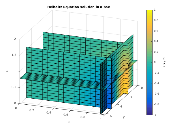
Example
This example solves the Helmholz equation
for
,
where
, and
is derived from the exact solution
The equation is subject to the following boundary conditions, again derived from the exact solution given above.
- and are prescribed (i.e., ).
- (i.e., ).
- and are prescribed (i.e., ).
Open in the MATLAB editor:
d03fa_example
function d03fa_example
fprintf('d03fa example results\n\n');
xs = 0; xf = 1; l = 16;
ys = 0; yf = 2*pi; m = 32;
zs = 0; zf = pi/2; n = 20;
bdxs = zeros(m+1, n+1); bdxf = zeros(m+1, n+1);
bdys = zeros(l+1, n+1); bdyf = zeros(l+1, n+1);
bdzs = zeros(l+1, m+1); bdzf = zeros(l+1, m+1);
lbdcnd = int64(1);
mbdcnd = int64(0);
nbdcnd = int64(2);
lambda = -2;
dx = (xf-xs)/l; x = [xs:dx:xf];
dy = (yf-ys)/m; y = [ys:dy:yf];
dz = (zf-zs)/n; z = [zs:dz:zf];
XY = [x.^4]'*sin(y);
bdzf = -XY;
YZ = [sin(y)]'*cos(z);
for i = 1:l
f(i,:,:) = (4*x(i)^2*(3-x(i)^2))*YZ;
g(i,:,:) = x(i)^4*YZ;
end
g(l+1,:,:) = YZ;
f(1,:,:) = 0;
f(l+1,:,:) = YZ;
f(:,:,1) = XY;
[u, pertrb, ifail] = d03fa( ...
xs, xf, int64(l), lbdcnd, bdxs, bdxf, ...
ys, yf, int64(m), mbdcnd, bdys, bdyf, ...
zs, zf, int64(n), nbdcnd, bdzs, bdzf, lambda, f);
maxerr = max(max(max(abs(u - g))));
fprintf('Maximum error in computed solution = %10.3e\n',maxerr);
fig1 = figure;
[xs,ys,zs] = meshgrid(y,x,z);
slice(xs,ys,zs,u,[1.8 5],[0.95],[0.78]);
axis([y(1) y(end) x(1) x(end) 0 2]);
xlabel('y'); ylabel('x'); zlabel('z');
title('Helholtz Equation solution in a box');
view(111, 26);
h = colorbar;
ylabel(h, 'u(x,y,z)')
d03fa example results

Maximum error in computed solution =  5.177e-04
PDF version (NAG web site
, 64-bit version, 64-bit version)
© The Numerical Algorithms Group Ltd, Oxford, UK. 2009–2015