PDF version (NAG web site
, 64-bit version, 64-bit version)
NAG Toolbox: nag_pde_1d_parab_keller (d03pe)
Purpose
nag_pde_1d_parab_keller (d03pe) integrates a system of linear or nonlinear, first-order, time-dependent partial differential equations (PDEs) in one space variable. The spatial discretization is performed using the Keller box scheme and the method of lines is employed to reduce the PDEs to a system of ordinary differential equations (ODEs). The resulting system is solved using a Backward Differentiation Formula (BDF) method.
Syntax
[
ts,
u,
rsave,
isave,
ind,
ifail] = d03pe(
ts,
tout,
pdedef,
bndary,
u,
x,
nleft,
acc,
rsave,
isave,
itask,
itrace,
ind, 'npde',
npde, 'npts',
npts)
[
ts,
u,
rsave,
isave,
ind,
ifail] = nag_pde_1d_parab_keller(
ts,
tout,
pdedef,
bndary,
u,
x,
nleft,
acc,
rsave,
isave,
itask,
itrace,
ind, 'npde',
npde, 'npts',
npts)
Note: the interface to this routine has changed since earlier releases of the toolbox:
| At Mark 22: |
lrsave and lisave were removed from the interface |
Description
nag_pde_1d_parab_keller (d03pe) integrates the system of first-order PDEs
In particular the functions
must have the general form
where
and
depend on
,
,
,
and the vector
is the set of solution values
and the vector
is its partial derivative with respect to
. Note that
and
must not depend on
.
The integration in time is from to , over the space interval , where and are the leftmost and rightmost points of a user-defined mesh . The mesh should be chosen in accordance with the expected behaviour of the solution.
The PDE system which is defined by the functions
must be specified in
pdedef.
The initial values of the functions
must be given at
. For a first-order system of PDEs, only one boundary condition is required for each PDE component
. The
npde boundary conditions are separated into
at the left-hand boundary
, and
at the right-hand boundary
, such that
. The position of the boundary condition for each component should be chosen with care; the general rule is that if the characteristic direction of
at the left-hand boundary (say) points into the interior of the solution domain, then the boundary condition for
should be specified at the left-hand boundary. Incorrect positioning of boundary conditions generally results in initialization or integration difficulties in the underlying time integration functions.
The boundary conditions have the form:
at the left-hand boundary, and
at the right-hand boundary.
Note that the functions
and
must not depend on
, since spatial derivatives are not determined explicitly in the Keller box scheme (see
Keller (1970)). If the problem involves derivative (Neumann) boundary conditions then it is generally possible to restate such boundary conditions in terms of permissible variables. Also note that
and
must be linear with respect to time derivatives, so that the boundary conditions have the general form
at the left-hand boundary, and
at the right-hand boundary, where
,
,
, and
depend on
,
and
only.
The boundary conditions must be specified in
bndary.
The problem is subject to the following restrictions:
| (i) |
, so that integration is in the forward direction; |
| (ii) |
and must not depend on any time derivatives; |
| (iii) |
The evaluation of the function is done at the mid-points of the mesh intervals by calling the pdedef for each mid-point in turn. Any discontinuities in the function must therefore be at one or more of the mesh points ; |
| (iv) |
At least one of the functions must be nonzero so that there is a time derivative present in the problem. |
In this method of lines approach the Keller box scheme (see
Keller (1970)) is applied to each PDE in the space variable only, resulting in a system of ODEs in time for the values of
at each mesh point. In total there are
ODEs in the time direction. This system is then integrated forwards in time using a BDF method.
References
Berzins M (1990) Developments in the NAG Library software for parabolic equations Scientific Software Systems (eds J C Mason and M G Cox) 59–72 Chapman and Hall
Berzins M, Dew P M and Furzeland R M (1989) Developing software for time-dependent problems using the method of lines and differential-algebraic integrators Appl. Numer. Math. 5 375–397
Keller H B (1970) A new difference scheme for parabolic problems Numerical Solutions of Partial Differential Equations (ed J Bramble) 2 327–350 Academic Press
Pennington S V and Berzins M (1994) New NAG Library software for first-order partial differential equations ACM Trans. Math. Softw. 20 63–99
Parameters
Compulsory Input Parameters
- 1:
– double scalar
-
The initial value of the independent variable .
Constraint:
.
- 2:
– double scalar
-
The final value of to which the integration is to be carried out.
- 3:
– function handle or string containing name of m-file
-
pdedef must compute the functions
which define the system of PDEs.
pdedef is called approximately midway between each pair of mesh points in turn by
nag_pde_1d_parab_keller (d03pe).
[res, ires] = pdedef(npde, t, x, u, ut, ux, ires)
Input Parameters
- 1:
– int64int32nag_int scalar
-
The number of PDEs in the system.
- 2:
– double scalar
-
The current value of the independent variable .
- 3:
– double scalar
-
The current value of the space variable .
- 4:
– double array
-
contains the value of the component , for .
- 5:
– double array
-
contains the value of the component , for .
- 6:
– double array
-
contains the value of the component , for .
- 7:
– int64int32nag_int scalar
-
The form of
that must be returned in the array
res.
- Equation (8) must be used.
- Equation (9) must be used.
- Indicates to the integrator that control should be passed back immediately to the calling (sub)routine with the error indicator set to .
- Indicates to the integrator that the current time step should be abandoned and a smaller time step used instead. You may wish to set when a physically meaningless input or output value has been generated. If you consecutively set , then nag_pde_1d_parab_keller (d03pe) returns to the calling function with the error indicator set to .
Output Parameters
- 1:
– double array
-
must contain the
th component of
, for
, where
is defined as
i.e., only terms depending explicitly on time derivatives, or
i.e., all terms in equation
(2).
The definition of
is determined by the input value of
ires.
- 2:
– int64int32nag_int scalar
-
Should usually remain unchanged. However, you may set
ires to force the integration function to take certain actions, as described below:
- Indicates to the integrator that control should be passed back immediately to the calling (sub)routine with the error indicator set to .
- Indicates to the integrator that the current time step should be abandoned and a smaller time step used instead. You may wish to set when a physically meaningless input or output value has been generated. If you consecutively set , then nag_pde_1d_parab_keller (d03pe) returns to the calling function with the error indicator set to .
- 4:
– function handle or string containing name of m-file
-
bndary must compute the functions
and
which define the boundary conditions as in equations
(4) and
(5).
[res, ires] = bndary(npde, t, ibnd, nobc, u, ut, ires)
Input Parameters
- 1:
– int64int32nag_int scalar
-
The number of PDEs in the system.
- 2:
– double scalar
-
The current value of the independent variable .
- 3:
– int64int32nag_int scalar
-
Determines the position of the boundary conditions.
- bndary must compute the left-hand boundary condition at .
- Indicates that bndary must compute the right-hand boundary condition at .
- 4:
– int64int32nag_int scalar
-
Specifies the number of boundary conditions at the boundary specified by
ibnd.
- 5:
– double array
-
contains the value of the component
at the boundary specified by
ibnd, for
.
- 6:
– double array
-
contains the value of the component
at the boundary specified by
ibnd, for
.
- 7:
– int64int32nag_int scalar
-
The form
(or
) that must be returned in the array
res.
- Equation (10) must be used.
- Equation (11) must be used.
Output Parameters
- 1:
– double array
-
must contain the
th component of
or
, depending on the value of
ibnd, for
, where
is defined as
i.e., only terms depending explicitly on time derivatives, or
i.e., all terms in equation
(6), and similarly for
.
The definitions of
and
are determined by the input value of
ires.
- 2:
– int64int32nag_int scalar
-
Should usually remain unchanged. However, you may set
ires to force the integration function to take certain actions, as described below:
- Indicates to the integrator that control should be passed back immediately to the calling (sub)routine with the error indicator set to .
- Indicates to the integrator that the current time step should be abandoned and a smaller time step used instead. You may wish to set when a physically meaningless input or output value has been generated. If you consecutively set , then nag_pde_1d_parab_keller (d03pe) returns to the calling function with the error indicator set to .
- 5:
– double array
-
The initial values of at and the mesh points
, for .
- 6:
– double array
-
The mesh points in the spatial direction. must specify the left-hand boundary, , and must specify the right-hand boundary, .
Constraint:
.
- 7:
– int64int32nag_int scalar
-
The number of boundary conditions at the left-hand mesh point .
Constraint:
.
- 8:
– double scalar
-
A positive quantity for controlling the local error estimate in the time integration. If
is the estimated error for
at the
th mesh point, the error test is:
Constraint:
.
- 9:
– double array
-
lrsave, the dimension of the array, must satisfy the constraint
.
If
,
rsave need not be set on entry.
If
,
rsave must be unchanged from the previous call to the function because it contains required information about the iteration.
- 10:
– int64int32nag_int array
-
lisave, the dimension of the array, must satisfy the constraint
.
If
,
isave need not be set on entry.
If
,
isave must be unchanged from the previous call to the function because it contains required information about the iteration. In particular:
- Contains the number of steps taken in time.
- Contains the number of residual evaluations of the resulting ODE system used. One such evaluation involves computing the PDE functions at all the mesh points, as well as one evaluation of the functions in the boundary conditions.
- Contains the number of Jacobian evaluations performed by the time integrator.
- Contains the order of the last backward differentiation formula method used.
- Contains the number of Newton iterations performed by the time integrator. Each iteration involves an ODE residual evaluation followed by a back-substitution using the decomposition of the Jacobian matrix.
- 11:
– int64int32nag_int scalar
-
Specifies the task to be performed by the ODE integrator.
- Normal computation of output values at .
- Take one step and return.
- Stop at the first internal integration point at or beyond .
Constraint:
, or .
- 12:
– int64int32nag_int scalar
-
The level of trace information required from
nag_pde_1d_parab_keller (d03pe) and the underlying ODE solver as follows:
- No output is generated.
- Only warning messages from the PDE solver are printed on the current error message unit (see nag_file_set_unit_error (x04aa)).
- Output from the underlying ODE solver is printed on the current advisory message unit (see nag_file_set_unit_advisory (x04ab)). This output contains details of Jacobian entries, the nonlinear iteration and the time integration during the computation of the ODE system.
- Output from the underlying ODE solver is similar to that produced when , except that the advisory messages are given in greater detail.
- Output from the underlying ODE solver is similar to that produced when , except that the advisory messages are given in greater detail.
You are advised to set
, unless you are experienced with
Sub-chapter D02M–N.
- 13:
– int64int32nag_int scalar
-
Indicates whether this is a continuation call or a new integration.
- Starts or restarts the integration in time.
- Continues the integration after an earlier exit from the function. In this case, only the arguments tout and ifail should be reset between calls to nag_pde_1d_parab_keller (d03pe).
Constraint:
or .
Optional Input Parameters
- 1:
– int64int32nag_int scalar
-
Default:
the first dimension of the array
u.
The number of PDEs in the system to be solved.
Constraint:
.
- 2:
– int64int32nag_int scalar
-
Default:
the dimension of the array
x and the second dimension of the array
u. (An error is raised if these dimensions are not equal.)
The number of mesh points in the interval .
Constraint:
.
Output Parameters
- 1:
– double scalar
-
The value of
corresponding to the solution values in
u. Normally
.
- 2:
– double array
-
will contain the computed solution at .
- 3:
– double array
-
If
,
rsave must be unchanged from the previous call to the function because it contains required information about the iteration.
- 4:
– int64int32nag_int array
-
If
,
isave must be unchanged from the previous call to the function because it contains required information about the iteration. In particular:
- Contains the number of steps taken in time.
- Contains the number of residual evaluations of the resulting ODE system used. One such evaluation involves computing the PDE functions at all the mesh points, as well as one evaluation of the functions in the boundary conditions.
- Contains the number of Jacobian evaluations performed by the time integrator.
- Contains the order of the last backward differentiation formula method used.
- Contains the number of Newton iterations performed by the time integrator. Each iteration involves an ODE residual evaluation followed by a back-substitution using the decomposition of the Jacobian matrix.
- 5:
– int64int32nag_int scalar
-
.
- 6:
– int64int32nag_int scalar
unless the function detects an error (see
Error Indicators and Warnings).
Error Indicators and Warnings
Errors or warnings detected by the function:
Cases prefixed with W are classified as warnings and
do not generate an error of type NAG:error_n. See nag_issue_warnings.
-
-
| On entry, | , |
| or | is too small, |
| or | , or , |
| or | are not ordered correctly, |
| or | , |
| or | , |
| or | nleft is not in the range to npde, |
| or | , |
| or | or , |
| or | lrsave is too small, |
| or | lisave is too small, |
| or | nag_pde_1d_parab_keller (d03pe) called initially with . |
- W
-
The underlying ODE solver cannot make any further progress across the integration range from the current point
with the supplied value of
acc. The components of
u contain the computed values at the current point
.
- W
-
In the underlying ODE solver, there were repeated errors or corrector convergence test failures on an attempted step, before completing the requested task. The problem may have a singularity or
acc is too small for the integration to continue. Incorrect positioning of boundary conditions may also result in this error. Integration was successful as far as
.
-
-
In setting up the ODE system, the internal initialization function was unable to initialize the derivative of the ODE system. This could be due to the fact that
ires was repeatedly set to
in the
pdedef or
bndary, when the residual in the underlying ODE solver was being evaluated. Incorrect positioning of boundary conditions may also result in this error.
-
-
In solving the ODE system, a singular Jacobian has been encountered. You should check their problem formulation.
- W
-
When evaluating the residual in solving the ODE system,
ires was set to
in one of
pdedef or
bndary. Integration was successful as far as
.
-
-
The value of
acc is so small that the function is unable to start the integration in time.
-
-
In either,
pdedef or
bndary,
ires was set to an invalid value.
- (nag_ode_ivp_stiff_imp_revcom (d02nn))
-
A serious error has occurred in an internal call to the specified function. Check the problem specification and all arguments and array dimensions. Setting
may provide more information. If the problem persists, contact
NAG.
- W
-
The required task has been completed, but it is estimated that a small change in
acc is unlikely to produce any change in the computed solution. (Only applies when you are not operating in one step mode, that is when
.)
-
-
An error occurred during Jacobian formulation of the ODE system (a more detailed error description may be directed to the current advisory message unit).
-
An unexpected error has been triggered by this routine. Please
contact
NAG.
-
Your licence key may have expired or may not have been installed correctly.
-
Dynamic memory allocation failed.
Accuracy
nag_pde_1d_parab_keller (d03pe) controls the accuracy of the integration in the time direction but not the accuracy of the approximation in space. The spatial accuracy depends on both the number of mesh points and on their distribution in space. In the time integration only the local error over a single step is controlled and so the accuracy over a number of steps cannot be guaranteed. You should therefore test the effect of varying the accuracy argument,
acc.
Further Comments
The Keller box scheme can be used to solve higher-order problems which have been reduced to first-order by the introduction of new variables (see the example problem in
nag_pde_1d_parab_dae_keller (d03pk)). In general, a second-order problem can be solved with slightly greater accuracy using the Keller box scheme instead of a finite difference scheme (
nag_pde_1d_parab_fd (d03pc) or
nag_pde_1d_parab_dae_fd (d03ph) for example), but at the expense of increased CPU time due to the larger number of function evaluations required.
It should be noted that the Keller box scheme, in common with other central-difference schemes, may be unsuitable for some hyperbolic first-order problems such as the apparently simple linear advection equation
, where
is a constant, resulting in spurious oscillations due to the lack of dissipation. This type of problem requires a discretization scheme with upwind weighting (
nag_pde_1d_parab_convdiff (d03pf) for example), or the addition of a second-order artificial dissipation term.
The time taken depends on the complexity of the system and on the accuracy requested.
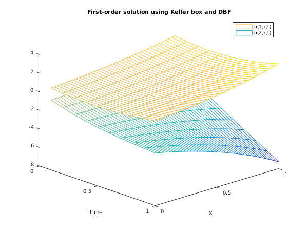
Example
This example is the simple first-order system
for
and
.
The initial conditions are
and the Dirichlet boundary conditions for
at
and
at
are given by the exact solution:
Open in the MATLAB editor:
d03pe_example
function d03pe_example
fprintf('d03pe example results\n\n');
ts = 0;
dx = 0.025;
x = [0:dx:1];
npts = 1 + 1/0.025;
u(1,1:npts) = exp(x);
u(2,1:npts) = sin(x);
nleft = int64(1);
acc = 1e-06;
rsave = zeros(4000, 1);
isave = zeros(200, 1, 'int64');
itask = int64(1);
itrace = int64(0);
ind = int64(0);
fprintf('%32s\n%6s ','x','t');
fprintf('%10.4f',x(5:8:37));
fprintf('\n');
pr = false;
i = 0;
t = [0.1:0.1:1];
for tout = t
i = i+1;
[ts, u, rsave, isave, ind, ifail] = ...
d03pe(...
ts, tout, @pdedef, @bndary, u, x, nleft, acc, ...
rsave, isave, itask, itrace, ind);
if pr
fprintf('%6.1f %3s',ts,'U1:');
fprintf('%10.4f',u(1,5:8:37));
fprintf('\n%10s','U2:');
fprintf('%10.4f',u(2,5:8:37));
fprintf('\n');
end
pr = ~pr;
v(:,i) = u(1,:);
w(:,i) = u(2,:);
end
fig1 = figure;
hold on
mesh(t,x,v);
mesh(t,x,w);
xlabel('Time');
ylabel('x');
title('First-order solution using Keller box and DBF');
legend('u(1,x,t)','u(2,x,t)');
view(47,26);
hold off
function [res, ires] = pdedef(npde, t, x, u, ut, ux, ires)
if (ires == -1)
res(1:2) = ut(1:2);
else
res(1) = ut(1) + ux(1) + ux(2);
res(2) = ut(2) + 4*ux(1) + ux(2);
end
function [res, ires] = bndary(npde, t, ibnd, nobc, u, ut, ires)
if (ibnd == 0)
if (ires == -1)
res(1) = 0;
else
res(1) = u(1) - (exp(t)+exp(-3*t))/2 - (sin(-3*t)-sin(t))/4;
end
else
if (ires == -1)
res(1) = 0;
else
res(1) = u(2) - exp(1-3*t) + exp(1+t) - (sin(1-3*t)+sin(1+t))/2;
end
end
d03pe example results

                               x
     t        0.1000    0.3000    0.5000    0.7000    0.9000
   0.2 U1:    0.7845    1.0010    1.2733    1.6115    2.0281
       U2:   -0.8352   -0.8159   -0.8367   -0.9128   -1.0609
   0.4 U1:    0.6481    0.8533    1.1212    1.4627    1.8903
       U2:   -1.5216   -1.6767   -1.8934   -2.1917   -2.5945
   0.6 U1:    0.6892    0.8961    1.1747    1.5374    1.9989
       U2:   -2.0047   -2.3434   -2.7677   -3.3002   -3.9680
   0.8 U1:    0.8977    1.1247    1.4320    1.8349    2.3513
       U2:   -2.3403   -2.8675   -3.5110   -4.2960   -5.2537
   1.0 U1:    1.2470    1.5205    1.8829    2.3528    2.9519
       U2:   -2.6229   -3.3338   -4.1999   -5.2506   -6.5218
PDF version (NAG web site
, 64-bit version, 64-bit version)
© The Numerical Algorithms Group Ltd, Oxford, UK. 2009–2015