hide long namesshow long names
hide short namesshow short names
Integer type:  int32  int64  nag_int  show int32  show int32  show int64  show int64  show nag_int  show nag_int

PDF version (NAG web site, 64-bit version, 64-bit version)
Chapter Contents
Chapter Introduction
NAG Toolbox

NAG Toolbox: nag_pde_1d_parab_coll_interp (d03py)

 Contents

    1  Purpose
    2  Syntax
    7  Accuracy
    9  Example

Purpose

nag_pde_1d_parab_coll_interp (d03py) may be used in conjunction with either nag_pde_1d_parab_coll (d03pd) or nag_pde_1d_parab_dae_coll (d03pj). It computes the solution and its first derivative at user-specified points in the spatial coordinate.

Syntax

[up, rsave, ifail] = d03py(u, xbkpts, npoly, xp, itype, rsave, 'npde', npde, 'nbkpts', nbkpts, 'npts', npts, 'intpts', intpts)
[up, rsave, ifail] = nag_pde_1d_parab_coll_interp(u, xbkpts, npoly, xp, itype, rsave, 'npde', npde, 'nbkpts', nbkpts, 'npts', npts, 'intpts', intpts)
Note: the interface to this routine has changed since earlier releases of the toolbox:
At Mark 22: lrsave was removed from the interface

Description

nag_pde_1d_parab_coll_interp (d03py) is an interpolation function for evaluating the solution of a system of partial differential equations (PDEs), or the PDE components of a system of PDEs with coupled ordinary differential equations (ODEs), at a set of user-specified points. The solution of a system of equations can be computed using nag_pde_1d_parab_coll (d03pd) or nag_pde_1d_parab_dae_coll (d03pj) on a set of mesh points; nag_pde_1d_parab_coll_interp (d03py) can then be employed to compute the solution at a set of points other than those originally used in nag_pde_1d_parab_coll (d03pd) or nag_pde_1d_parab_dae_coll (d03pj). It can also evaluate the first derivative of the solution. Polynomial interpolation is used between each of the break-points xbkptsi, for i=1,2,,nbkpts. When the derivative is needed (itype=2), the array xpintpts must not contain any of the break-points, as the method, and consequently the interpolation scheme, assumes that only the solution is continuous at these points.

References

None.

Parameters

Note: the arguments u, npts, npde, xbkpts, nbkpts, rsave and lrsave must be supplied unchanged from either nag_pde_1d_parab_coll (d03pd) or nag_pde_1d_parab_dae_coll (d03pj).

Compulsory Input Parameters

1:     unpdenpts – double array
The PDE part of the original solution returned in the argument u by the function nag_pde_1d_parab_coll (d03pd) or nag_pde_1d_parab_dae_coll (d03pj).
2:     xbkptsnbkpts – double array
xbkptsi, for i=1,2,,nbkpts, must contain the break-points as used by nag_pde_1d_parab_coll (d03pd) or nag_pde_1d_parab_dae_coll (d03pj).
Constraint: xbkpts1<xbkpts2<<xbkptsnbkpts.
3:     npoly int64int32nag_int scalar
The degree of the Chebyshev polynomial used for approximation as used by nag_pde_1d_parab_coll (d03pd) or nag_pde_1d_parab_dae_coll (d03pj).
Constraint: 1npoly49.
4:     xpintpts – double array
xpi, for i=1,2,,intpts, must contain the spatial interpolation points.
Constraints:
  • xbkpts1xp1<xp2<<xpintptsxbkptsnbkpts;
  • if itype=2, xpixbkptsj, for i=1,2,,intpts and j=2,3,,nbkpts-1.
5:     itype int64int32nag_int scalar
Specifies the interpolation to be performed.
itype=1
The solution at the interpolation points are computed.
itype=2
Both the solution and the first derivative at the interpolation points are computed.
Constraint: itype=1 or 2.
6:     rsavelrsave – double array
The array rsave contains information required by nag_pde_1d_parab_coll_interp (d03py) as returned by nag_pde_1d_parab_coll (d03pd) or nag_pde_1d_parab_dae_coll (d03pj). The contents of rsave must not be changed from the call to nag_pde_1d_parab_coll (d03pd) or nag_pde_1d_parab_dae_coll (d03pj). Some elements of this array are overwritten on exit.

Optional Input Parameters

1:     npde int64int32nag_int scalar
Default: the first dimension of the array u.
The number of PDEs.
Constraint: npde1.
2:     nbkpts int64int32nag_int scalar
Default: the dimension of the array xbkpts.
The number of break-points.
Constraint: nbkpts2.
3:     npts int64int32nag_int scalar
Default: the second dimension of the array u.
The number of mesh points as used by nag_pde_1d_parab_coll (d03pd) or nag_pde_1d_parab_dae_coll (d03pj).
Constraint: npts=nbkpts-1×npoly+1.
4:     intpts int64int32nag_int scalar
Default: the dimension of the array xp.
The number of interpolation points.
Constraint: intpts1.

Output Parameters

1:     upnpdeintptsitype – double array
If itype=1, upij1, contains the value of the solution Uixj,tout, at the interpolation points xj=xpj, for j=1,2,,intpts and i=1,2,,npde.
If itype=2, upij1 contains Uixj,tout and upij2 contains Ui x at these points.
2:     rsavelrsave – double array
3:     ifail int64int32nag_int scalar
ifail=0 unless the function detects an error (see Error Indicators and Warnings).

Error Indicators and Warnings

Errors or warnings detected by the function:
   ifail=1
On entry,itype1 or 2,
ornpoly<1,
ornpde<1,
ornbkpts<2,
orintpts<1,
ornptsnbkpts-1×npoly+1,
or xbkptsi, for i=1,2,,nbkpts, are not ordered.
   ifail=2
On entry, the interpolation points xpi, for i=1,2,,intpts, are not in strictly increasing order, or when itype=2, at least one of the interpolation points stored in xp is equal to one of the break-points stored in xbkpts.
   ifail=3
You are attempting extrapolation, that is, one of the interpolation points xpi, for some i, lies outside the interval [xbkpts1,xbkptsnbkpts]. Extrapolation is not permitted.
   ifail=-99
An unexpected error has been triggered by this routine. Please contact NAG.
   ifail=-399
Your licence key may have expired or may not have been installed correctly.
   ifail=-999
Dynamic memory allocation failed.

Accuracy

See the documents for nag_pde_1d_parab_coll (d03pd) or nag_pde_1d_parab_dae_coll (d03pj).

Further Comments

None.

Example

See Example in nag_pde_1d_parab_coll (d03pd).
function d03py_example


fprintf('d03py example results\n\n');

% Solution of an elliptic-parabolic pair of PDEs
% (derived from a fourth-order PDE).

% Set values for problem parameters.
npde = 2;

% Number of points on interpolated mesh, number of break points.
intpts = 6;
nbkpts = 10;

% Order of Chebyshev polynomial.
npoly = int64(3);

npts   = (nbkpts-1)*npoly + 1;
lisave = npde*npts + 24;

% Define some arrays.
rsave   = zeros(4000, 1);
u       = zeros(npde, npts);
isave   = zeros(lisave, 1, 'int64');
lwsav   = false(100, 1);
iwsav   = zeros(505, 1, 'int64');
rwsav   = zeros(1100, 1);
cwsav   = {''; ''; ''; ''; ''; ''; ''; ''; ''; ''};
% Set up the points on the interpolation grid.
xinterp = [-1:0.4:1];


% Number of output points in time.
niter  = 20;

% Prepare to store plotting results.
tsav   = zeros(niter, 1);
usav   = zeros(2, niter, npts);
isav   = 0;

% Set the break points.
hx     = 2/(nbkpts-1);
xbkpts = [-1:hx:1];

% Set initial conditions.
m      = int64(0);
ts     = 0.0;
tout   = 0.1e-4;
acc    = 1.0e-4;
itask  = int64(1);
itrace = int64(0);
ind0   = int64(0);

alpha  = -log(tout)/(niter-1);

% Output algorithmic details and interpolation points.
fprintf('polynomial degree = %4d    no. of elements = %4d\n', npoly, nbkpts-1);
fprintf('accuracy requirement = %10.3e    number of points = %5d', acc, npts);
fprintf('\n\n t / x       ');
fprintf('%8.4f', xinterp);
fprintf('\n\n');

% Loop over exponentially increasing endpoints of integration 0.0001 --> 1. 
% Set itask = 1: normal computation of output values at t = tout.
for iter = 1:niter

  tout = exp(alpha*(iter - niter));

  % (re)start integration in time: ind0=0.
  [ts, u, x, rsave, isave, ind, user, cwsav, lwsav, iwsav, rwsav, ifail] = ...
  d03pd( ...
         m, ts, tout, @pdedef, ...
         @bndary, u, xbkpts, npoly, @uinit, ...
         acc, rsave, isave, itask, itrace, ind0, ...
         cwsav, lwsav, iwsav, rwsav);

  % Interpolation onto coarser grid for display
  itype  = int64(1);
  [uinterp, rsave, ifail] = d03py( ...
                                   u, xbkpts, npoly, xinterp, itype, rsave);

  % Output interpolated results for this time step.
  fprintf('%7.4f  u(1)', ts);
  fprintf('%8.4f', uinterp(1,:,1));
  fprintf('\n         u(2)');
  fprintf('%8.4f', uinterp(2,:,1));
  fprintf('\n\n');

  % Save this timestep for plotting.
  isav = isav+1;
  tsav(isav) = ts;
  usav(1:2,isav,1:npts) = u(1:2,1:npts);
end

% Output some statistics.
fprintf(' Number of integration steps in time = %6d\n', isave(1));
fprintf(' Number of function evaluations      = %6d\n', isave(2));
fprintf(' Number of Jacobian evaluations      = %6d\n', isave(3));
fprintf(' Number of iterations                = %6d\n', isave(5));
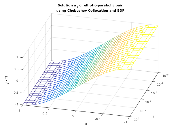
% Plot results.
fig1 = figure;
plot_results(x, tsav, squeeze(usav(1,:,:)), 'u_1');
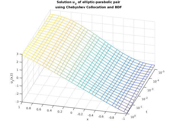
fig2 = figure;
plot_results(x, tsav, squeeze(usav(2,:,:)), 'u_2');


function [p, q, r, ires, user] = pdedef(npde, t, x, nptl, u, ux, ires, user)
  p = zeros(npde, npde, nptl);
  q = zeros(npde, nptl);
  r = zeros(npde, nptl);

  for i = 1:double(nptl)
    q(1,i) = u(2,i);
    q(2,i) = u(1,i)*ux(2,i) - ux(1,i)*u(2,i);
    r(1,i) = ux(1,i);
    r(2,i) = ux(2,i);
    p(2,2,i) = 1;
  end;


function [beta, gamma, ires, user] = bndary(npde, t, u, ux, ibnd, ires, user)
  beta  = zeros(npde, 1);
  gamma = zeros(npde, 1);

  beta(1)  = 1;
  beta(2)  = 0;
  gamma(1) = 0;
  if (ibnd == 0)
    gamma(2) = u(1) - 1;
  else
    gamma(2) = u(1) + 1;
  end


function [u, user] = uinit(npde, npts, x, user)
  u = zeros(npde, npts);

  piby2 = pi/2;
  u(1,:) = -sin(piby2*x);
  u(2,:) = -piby2*piby2*u(1,:);


function plot_results(x, t, u, ident)
  % Plot array as a mesh.
  mesh(x, t, u);
  set(gca, 'YScale', 'log');
  set(gca, 'YTick', [0.00001 0.0001 0.001 0.01 0.1 1]);
  set(gca, 'YMinorGrid', 'off');
  set(gca, 'YMinorTick', 'off');

  % Label the axes, and set the title.
  xlabel('x');
  ylabel('t');
  zlabel([ident,'(x,t)']);
  title({['Solution ',ident,' of elliptic-parabolic pair'], ...
      'using Chebyshev Collocation and BDF'});

  % Set the axes limits tight to the x and y range.
  axis([x(1) x(end) t(1) t(end)]);

  % Set the view to something nice (determined empirically).
  view(-165, 44);
d03py example results

polynomial degree =    3    no. of elements =    9
accuracy requirement =  1.000e-04    number of points =    28

 t / x        -1.0000 -0.6000 -0.2000  0.2000  0.6000  1.0000

 0.0000  u(1)  1.0000  0.8090  0.3090 -0.3090 -0.8090 -1.0000
         u(2) -2.4690 -1.9961 -0.7624  0.7624  1.9961  2.4690

 0.0000  u(1)  1.0000  0.8090  0.3090 -0.3090 -0.8090 -1.0000
         u(2) -2.4687 -1.9961 -0.7624  0.7624  1.9961  2.4687

 0.0000  u(1)  1.0000  0.8090  0.3090 -0.3090 -0.8090 -1.0000
         u(2) -2.4700 -1.9961 -0.7624  0.7624  1.9961  2.4700

 0.0001  u(1)  1.0000  0.8090  0.3090 -0.3090 -0.8090 -1.0000
         u(2) -2.4724 -1.9960 -0.7624  0.7624  1.9960  2.4724

 0.0001  u(1)  1.0000  0.8090  0.3090 -0.3090 -0.8090 -1.0000
         u(2) -2.4767 -1.9959 -0.7624  0.7624  1.9959  2.4767

 0.0002  u(1)  1.0000  0.8090  0.3090 -0.3090 -0.8090 -1.0000
         u(2) -2.4840 -1.9957 -0.7623  0.7623  1.9957  2.4840

 0.0004  u(1)  1.0000  0.8089  0.3090 -0.3090 -0.8089 -1.0000
         u(2) -2.4960 -1.9953 -0.7621  0.7621  1.9953  2.4960

 0.0007  u(1)  1.0000  0.8089  0.3089 -0.3089 -0.8089 -1.0000
         u(2) -2.5142 -1.9946 -0.7619  0.7619  1.9946  2.5142

 0.0013  u(1)  1.0000  0.8087  0.3089 -0.3089 -0.8087 -1.0000
         u(2) -2.5374 -1.9933 -0.7614  0.7614  1.9933  2.5374

 0.0023  u(1)  1.0000  0.8085  0.3087 -0.3087 -0.8085 -1.0000
         u(2) -2.5611 -1.9910 -0.7605  0.7605  1.9910  2.5611

 0.0043  u(1)  1.0000  0.8081  0.3085 -0.3085 -0.8081 -1.0000
         u(2) -2.5869 -1.9866 -0.7588  0.7588  1.9866  2.5869

 0.0078  u(1)  1.0000  0.8074  0.3081 -0.3081 -0.8074 -1.0000
         u(2) -2.6183 -1.9787 -0.7558  0.7558  1.9787  2.6183

 0.0144  u(1)  1.0000  0.8063  0.3075 -0.3075 -0.8063 -1.0000
         u(2) -2.6604 -1.9643 -0.7503  0.7503  1.9643  2.6604

 0.0264  u(1)  1.0000  0.8045  0.3064 -0.3064 -0.8045 -1.0000
         u(2) -2.7128 -1.9394 -0.7402  0.7402  1.9394  2.7128

 0.0483  u(1)  1.0000  0.8020  0.3046 -0.3046 -0.8020 -1.0000
         u(2) -2.7723 -1.9042 -0.7222  0.7222  1.9042  2.7723

 0.0886  u(1)  1.0000  0.7990  0.3022 -0.3022 -0.7990 -1.0000
         u(2) -2.8331 -1.8684 -0.6915  0.6915  1.8684  2.8331

 0.1624  u(1)  1.0000  0.7962  0.2996 -0.2996 -0.7962 -1.0000
         u(2) -2.8840 -1.8423 -0.6512  0.6512  1.8423  2.8840

 0.2976  u(1)  1.0000  0.7944  0.2978 -0.2978 -0.7944 -1.0000
         u(2) -2.9140 -1.8287 -0.6218  0.6218  1.8287  2.9140

 0.5456  u(1)  1.0000  0.7939  0.2973 -0.2973 -0.7939 -1.0000
         u(2) -2.9225 -1.8250 -0.6129  0.6129  1.8250  2.9225

 1.0000  u(1)  1.0000  0.7939  0.2972 -0.2972 -0.7939 -1.0000
         u(2) -2.9233 -1.8247 -0.6120  0.6120  1.8247  2.9233

 Number of integration steps in time =     38
 Number of function evaluations      =    237
 Number of Jacobian evaluations      =      9
 Number of iterations                =     89
d03py_fig1.png
d03py_fig2.png

PDF version (NAG web site, 64-bit version, 64-bit version)
Chapter Contents
Chapter Introduction
NAG Toolbox

© The Numerical Algorithms Group Ltd, Oxford, UK. 2009–2015