PDF version (NAG web site
, 64-bit version, 64-bit version)
NAG Toolbox: nag_tsa_uni_autocorr_part (g13ac)
Purpose
nag_tsa_uni_autocorr_part (g13ac) calculates partial autocorrelation coefficients given a set of autocorrelation coefficients. It also calculates the predictor error variance ratios for increasing order of finite lag autoregressive predictor, and the autoregressive parameters associated with the predictor of maximum order.
Syntax
Description
The data consist of values of autocorrelation coefficients
, relating to lags
. These will generally (but not necessarily) be sample values such as may be obtained from a time series
using
nag_tsa_uni_autocorr (g13ab).
The partial autocorrelation coefficient at lag
may be identified with the parameter
in the autoregression
where
is the predictor error.
The first subscript of and emphasizes the fact that the parameters will in general alter as further terms are introduced into the equation (i.e., as is increased).
The parameters are determined from the autocorrelation coefficients by the Yule–Walker equations
taking
when
, and
.
The predictor error variance ratio
is defined by
The above sets of equations are solved by a recursive method (the Durbin–Levinson algorithm). The recursive cycle applied for , where is the number of partial autocorrelation coefficients required, is initialized by setting and .
If the condition
occurs, say when
, it indicates that the supplied autocorrelation coefficients do not form a positive definite sequence (see
Hannan (1960)), and the recursion is not continued. The autoregressive parameters are overwritten at each recursive step, so that upon completion the only available values are
, for
, or
if the recursion has been prematurely halted.
References
Box G E P and Jenkins G M (1976) Time Series Analysis: Forecasting and Control (Revised Edition) Holden–Day
Durbin J (1960) The fitting of time series models Rev. Inst. Internat. Stat. 28 233
Hannan E J (1960) Time Series Analysis Methuen
Parameters
Compulsory Input Parameters
- 1:
– double array
-
The autocorrelation coefficient relating to lag
, for .
- 2:
– int64int32nag_int scalar
-
, the number of partial autocorrelation coefficients required.
Constraint:
.
Optional Input Parameters
- 1:
– int64int32nag_int scalar
-
Default:
the dimension of the array
r.
, the number of lags. The lags range from to and do not include zero.
Constraint:
.
Output Parameters
- 1:
– double array
-
contains the partial autocorrelation coefficient at lag , , for .
- 2:
– double array
-
contains the predictor error variance ratio , for .
- 3:
– double array
-
The autoregressive parameters of maximum order, i.e.,
if , or if , for .
- 4:
– int64int32nag_int scalar
-
The number of valid values in each of
p,
v and
ar. Thus in the case of premature termination at iteration
(see
Description),
nvl is returned as
.
- 5:
– int64int32nag_int scalar
unless the function detects an error (see
Error Indicators and Warnings).
Error Indicators and Warnings
Errors or warnings detected by the function:
Cases prefixed with W are classified as warnings and
do not generate an error of type NAG:error_n. See nag_issue_warnings.
-
-
| On entry, | , |
| or | , |
| or | . |
-
-
On entry, the autocorrelation coefficient of lag has an absolute value greater than or equal to ; no recursions could be performed.
- W
-
Recursion has been prematurely terminated; the supplied autocorrelation coefficients do not form a positive definite sequence (see
Description). Argument
nvl returns the number of valid values computed.
-
An unexpected error has been triggered by this routine. Please
contact
NAG.
-
Your licence key may have expired or may not have been installed correctly.
-
Dynamic memory allocation failed.
Accuracy
The computations are believed to be stable.
Further Comments
The time taken by nag_tsa_uni_autocorr_part (g13ac) is proportional to .
Example
This example uses an input series of
sample autocorrelation coefficients derived from the original series of sunspot numbers generated by the
nag_tsa_uni_autocorr (g13ab) example program. The results show five values of each of the three output arrays: partial autocorrelation coefficients, predictor error variance ratios and autoregressive parameters. All of these were valid.
Open in the MATLAB editor:
g13ac_example
function g13ac_example
fprintf('g13ac example results\n\n');
r = [ 0.8004 0.4355 0.0328 -0.2835 -0.4505 ...
-0.4242 -0.2419 0.0550 0.3783 0.5857 ...
0.6123 0.4389 0.1538 -0.1626 -0.3828 ...
-0.4637 -0.4133 -0.2630 -0.0711 0.1217 ...
0.2547 0.2681 0.1211 -0.0683 -0.2248 ...
-0.3187 -0.3365 -0.2748 -0.1696 -0.0500 ...
0.0605 0.1131 0.1132 0.0604 -0.0171 ...
-0.0909 -0.1269 -0.1345 -0.1056 -0.0581 ...
-0.0119 0.0272 0.0496 0.0592 0.0167 ...
-0.0138 -0.0328 -0.0383 -0.0287];
nl = int64(5);
[p, v, ar, nvl, ifail] = g13ac( ...
r, nl, 'nk', int64(10));
fprintf('Lag Partial Predictor error Autoregressive\n');
fprintf(' autocorrn variance ratio parameter\n\n');
ivar = double([1:nvl])';
fprintf('%2d%9.3f%16.3f%14.3f\n',[ivar p v ar]');
nl = int64(numel(r));
[p, v, ar, nvl, ifail] = g13ac( ...
r, nl);
fig1 = figure;
refline = 1.96/sqrt(50);
hold on
h = bar(p,0.1);
h.FaceColor = [1 0 0];
h.EdgeColor = [1 0 0];
h.ShowBaseLine = 'off';
plot([0 50],[refline refline],'green');
plot([0 50],[-refline -refline],'green');
axis([0 50 -0.6 1]);
ax = gca;
ax.YTick = [-0.6:0.2:1];
ax.XTick = [0:10:50];
xlabel('Lag');
ylabel('PACF');
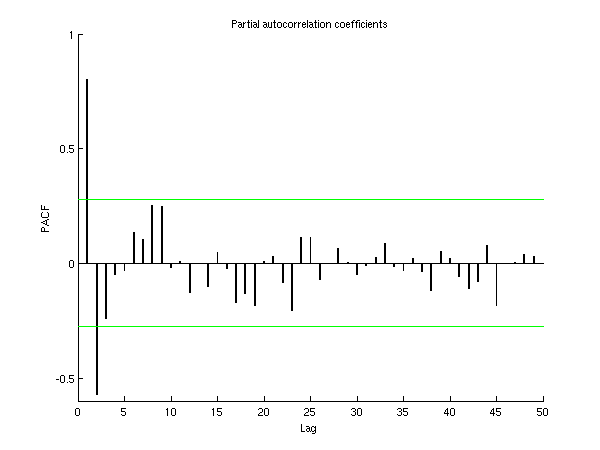
title('Partial autocorrelation coefficients');
hold off
g13ac example results

Lag  Partial    Predictor error  Autoregressive
     autocorrn  variance ratio   parameter

 1    0.800           0.359         1.108
 2   -0.571           0.242        -0.290
 3   -0.239           0.228        -0.193
 4   -0.049           0.228        -0.014
 5   -0.032           0.228        -0.032
This plot shows the partial autocorrelations for all possible lag values. Reference lines are given at .
PDF version (NAG web site
, 64-bit version, 64-bit version)
© The Numerical Algorithms Group Ltd, Oxford, UK. 2009–2015