PDF version (NAG web site
, 64-bit version, 64-bit version)
NAG Toolbox: nag_tsa_inhom_iema (g13me)
Purpose
nag_tsa_inhom_iema (g13me) calculates the iterated exponential moving average for an inhomogeneous time series.
Syntax
[
iema,
pn,
rcomm,
ifail] = g13me(
iema,
t,
tau,
m,
sinit,
inter, 'nb',
nb, 'pn',
pn, 'rcomm',
rcomm)
[
iema,
pn,
rcomm,
ifail] = nag_tsa_inhom_iema(
iema,
t,
tau,
m,
sinit,
inter, 'nb',
nb, 'pn',
pn, 'rcomm',
rcomm)
Description
nag_tsa_inhom_iema (g13me) calculates the iterated exponential moving average for an inhomogeneous time series. The time series is represented by two vectors of length ; a vector of times, ; and a vector of values, . Each element of the time series is therefore composed of the pair of scalar values , for . Time can be measured in any arbitrary units, as long as all elements of use the same units.
The exponential moving average (EMA), with parameter
, is an average operator, with the exponentially decaying kernel given by
The exponential form of this kernel gives rise to the following iterative formula for the EMA operator (see
Zumbach and Müller (2001)):
where
The value of
depends on the method of interpolation chosen.
nag_tsa_inhom_iema (g13me) gives the option of three interpolation methods:
| 1. |
Previous point: |
; |
| 2. |
Linear: |
; |
| 3. |
Next point: |
. |
The
-iterated exponential moving average,
,
, is defined using the recursive formula:
with
For large datasets or where all the data is not available at the same time, and can be split into arbitrary sized blocks and nag_tsa_inhom_iema (g13me) called multiple times.
References
Dacorogna M M, Gencay R, Müller U, Olsen R B and Pictet O V (2001) An Introduction to High-frequency Finance Academic Press
Zumbach G O and Müller U A (2001) Operators on inhomogeneous time series International Journal of Theoretical and Applied Finance 4(1) 147–178
Parameters
Compulsory Input Parameters
- 1:
– double array
-
, the current block of observations, for
, where
is the number of observations processed so far, i.e., the value supplied in
pn on entry.
- 2:
– double array
-
, the times for the current block of observations, for
, where
is the number of observations processed so far, i.e., the value supplied in
pn on entry.
If , will be returned, but nag_tsa_inhom_iema (g13me) will continue as if was strictly increasing by using the absolute value.
- 3:
– double scalar
-
, the argument controlling the rate of decay, which must be sufficiently large that , can be calculated without overflowing, for all .
Constraint:
.
- 4:
– int64int32nag_int scalar
-
, the number of times the EMA operator is to be iterated.
Constraint:
.
- 5:
– double array
-
If
, the values used to start the iterative process, with
- ,
- ,
- , for .
If
,
sinit is not referenced.
- 6:
– int64int32nag_int array
-
The type of interpolation used with
indicating the interpolation method to use when calculating
and
the interpolation method to use when calculating
,
.
Three types of interpolation are possible:
- Previous point, with .
- Linear, with .
- Next point, .
Zumbach and Müller (2001) recommend that linear interpolation is used in second and subsequent iterations, i.e.,
, irrespective of the interpolation method used at the first iteration, i.e., the value of
.
Constraint:
, or , for .
Optional Input Parameters
- 1:
– int64int32nag_int scalar
-
Default:
the dimension of the arrays
iema,
t. (An error is raised if these dimensions are not equal.)
, the number of observations in the current block of data. The size of the block of data supplied in
iema and
t can vary; therefore
nb can change between calls to
nag_tsa_inhom_iema (g13me).
Constraint:
.
- 2:
– int64int32nag_int scalar
Default:
, the number of observations processed so far. On the first call to
nag_tsa_inhom_iema (g13me), or when starting to summarise a new dataset,
pn must be set to
. On subsequent calls it must be the same value as returned by the last call to
nag_tsa_inhom_iema (g13me).
Constraint:
.
- 3:
– double array
Communication array, used to store information between calls to
nag_tsa_inhom_iema (g13me).
On the first call to
nag_tsa_inhom_iema (g13me), or if all the data is provided in one go,
rcomm need not be provided.
Output Parameters
- 1:
– double array
-
The iterated EMA, with .
- 2:
– int64int32nag_int scalar
Default:
, the updated number of observations processed so far.
- 3:
– double array
Communication array, used to store information between calls to nag_tsa_inhom_iema (g13me).
- 4:
– int64int32nag_int scalar
unless the function detects an error (see
Error Indicators and Warnings).
Error Indicators and Warnings
Errors or warnings detected by the function:
Cases prefixed with W are classified as warnings and
do not generate an error of type NAG:error_n. See nag_issue_warnings.
-
-
Constraint: .
- W
-
Constraint:
t should be strictly increasing.
-
-
Constraint: if linear interpolation is being used.
-
-
Constraint: .
-
-
Constraint: if
then
tau must be unchanged since previous call.
-
-
Constraint: .
-
-
Constraint: if
then
m must be unchanged since previous call.
-
-
Constraint: , or .
-
-
Constraint: , or .
-
-
Constraint: if
,
inter must be unchanged since the previous call.
-
-
Constraint: .
-
-
Constraint: if
then
pn must be unchanged since previous call.
-
-
rcomm has been corrupted between calls.
-
-
Constraint: if , or .
-
-
Constraint: if , .
- W
-
Truncation occurred to avoid overflow, check for extreme values in
t,
iema or for
tau. Results are returned using the truncated values.
-
An unexpected error has been triggered by this routine. Please
contact
NAG.
-
Your licence key may have expired or may not have been installed correctly.
-
Dynamic memory allocation failed.
Accuracy
Not applicable.
Further Comments
Approximately real elements are internally allocated by nag_tsa_inhom_iema (g13me).
The more data you supply to
nag_tsa_inhom_iema (g13me) in one call, i.e., the larger
nb is, the more efficient the function will be, particularly if the function is being run using more than one thread.
Checks are made during the calculation of
to avoid overflow. If a potential overflow is detected the offending value is replaced with a large positive or negative value, as appropriate, and the calculations performed based on the replacement values. In such cases
is returned. This should not occur in standard usage and will only occur if extreme values of
iema,
t or
tau are supplied.
Example
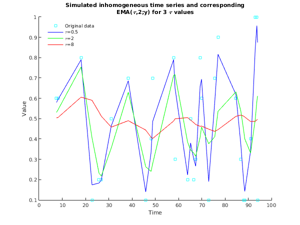
The example reads in a simulated time series, and calculates the iterated exponential moving average.
Open in the MATLAB editor:
g13me_example
function g13me_example
fprintf('g13me example results\n\n');
m = int64(2);
inter = [int64(3); 2];
tau = [0.5; 2; 8];
sinit = [5; 0.5; 0.5; 0.5];
nb = [5, 10, 15];
t = cell(3, 1);
iema = cell(3, 1);
t{1} = [ 7.5; 8.2; 18.1; 22.8; 25.8];
iema{1} = [ 0.6; 0.6; 0.8; 0.1; 0.2];
t{2} = [26.8; 31.1; 38.4; 45.9; 48.2; 48.9; 57.9; 58.5; 63.9; 65.2];
iema{2} = [ 0.2; 0.5; 0.7; 0.1; 0.4; 0.7; 0.8; 0.3; 0.2; 0.5];
t{3} = [66.6; 67.4; 69.3; 69.9; 73.0; 75.6; 77.0; 84.7; 86.8; 88.0; ...
88.5; 91.0; 93.0; 93.7; 94.0];
iema{3} = [ 0.2; 0.3; 0.8; 0.6; 0.1; 0.7; 0.9; 0.6; 0.3; 0.1; ...
0.1; 0.4; 1.0; 1.0; 0.1];
fprintf(' Time Iterated EMA\n');
fig1 = figure;
hold on
linecol = {'blue','green','red'};
xlabel('Time');
ylabel('Value');
title({'Simulated inhomogeneous time series and corresponding',
'EMA(\tau,2;y) for 3 \tau values'});
tm = [t{1}; t{2}; t{3}];
jm = [iema{1}; iema{2}; iema{3}];
plot(tm,jm,'cs');
for k = 1:numel(tau);
for i = 1:numel(nb)
if i == 1
[ema, pn, rcomm, ifail] = ...
g13me( ...
iema{i}, t{i}, tau(k), m, sinit, inter, 'rcomm', zeros(22,1));
jm = ema;
else
[ema, pn, rcomm, ifail] = ...
g13me( ...
iema{i}, t{i}, tau(k), m, sinit, inter, 'pn', pn, 'rcomm', rcomm);
jm = [jm; ema];
end
if k==2
for l=1:nb(i)
fprintf('%3d %10.1f %10.3f\n', pn-nb(i)+l, t{i}(l), ema(l));
end
fprintf('\n');
end
end
plot(tm,jm,linecol{k});
end
legend('Original data', '\tau=0.5', '\tau=2', '\tau=8', ...
'Location', 'northwest');
legend('boxoff');
hold off
g13me example results

             Time       Iterated EMA
  1           7.5         0.531
  2           8.2         0.544
  3          18.1         0.754
  4          22.8         0.406
  5          25.8         0.232

  6          26.8         0.217
  7          31.1         0.357
  8          38.4         0.630
  9          45.9         0.263
 10          48.2         0.241
 11          48.9         0.279
 12          57.9         0.713
 13          58.5         0.717
 14          63.9         0.385
 15          65.2         0.346

 16          66.6         0.330
 17          67.4         0.315
 18          69.3         0.409
 19          69.9         0.459
 20          73.0         0.377
 21          75.6         0.411
 22          77.0         0.536
 23          84.7         0.632
 24          86.8         0.538
 25          88.0         0.444
 26          88.5         0.401
 27          91.0         0.331
 28          93.0         0.495
 29          93.7         0.585
 30          94.0         0.612
This example plot shows the exponential moving average for the same data using three different values of and illustrates the effect on the EMA of altering this argument.
PDF version (NAG web site
, 64-bit version, 64-bit version)
© The Numerical Algorithms Group Ltd, Oxford, UK. 2009–2015