nag_tsa_cp_binary (g13nd) detects change points in a univariate time series, that is, the time points at which some feature of the data, for example the mean, changes. Change points are detected using binary segmentation using one of a provided set of cost functions.

Syntax

[tau, sparam, ifail] = g13nd(ctype, y, 'n', n, 'beta', beta, 'minss', minss, 'param', param, 'mdepth', mdepth)

[tau, sparam, ifail] = nag_tsa_cp_binary(ctype, y, 'n', n, 'beta', beta, 'minss', minss, 'param', param, 'mdepth', mdepth)

Description

Let

y_{1 : n} = \{y_{j} : j = 1, 2, \dots, n\}

denote a series of data and

τ = \{τ_{i} : i = 1, 2, \dots, m\}

denote a set of

m

ordered (strictly monotonic increasing) indices known as change points, with

1 \leq τ_{i} \leq n

and

τ_{m} = n

. For ease of notation we also define

τ_{0} = 0

. The

m

change points,

τ

, split the data into

m

segments, with the

i

th segment being of length

n_{i}

and containing

y_{τ_{i - 1} + 1 : τ_{i}}

Given a cost function,

C (y_{τ_{i - 1} + 1 : τ_{i}})

, nag_tsa_cp_binary (g13nd) gives an approximate solution to

\underset{m, τ}{minimize} \sum_{i = 1}^{m} (C (y_{τ_{i - 1} + 1 : τ_{i}}) + β)

where

β

is a penalty term used to control the number of change points. The solution is obtained in an iterative manner as follows:

Set

u = 1

w = n

and

k = 0

Set

k = k + 1

. If

k > K

, where

K

is a user-supplied control parameter, then terminate the process for this segment.

Find

v

that minimizes

C (y_{u : v}) + C (y_{v + 1 : w})

Test

C (y_{u : v}) + C (y_{v + 1 : w}) + β < C (y_{u : w})

(1)

If inequality (1) is false then the process is terminated for this segment.

If inequality (1) is true, then

v

is added to the set of change points, and the segment is split into two subsegments,

y_{u : v}

and

y_{v + 1 : w}

. The whole process is repeated from step 2 independently on each subsegment, with the relevant changes to the definition of

u

and

w

(i.e.,

w

is set to

v

when processing the left hand subsegment and

u

is set to

v + 1

when processing the right hand subsegment.

The change points are ordered to give

τ

nag_tsa_cp_binary (g13nd) supplies four families of cost function. Each cost function assumes that the series,

y

, comes from some distribution,

D (Θ)

. The parameter space,

Θ = \{θ, ϕ\}

is subdivided into

θ

containing those parameters allowed to differ in each segment and

ϕ

those parameters treated as constant across all segments. All four cost functions can then be described in terms of the likelihood function,

L

and are given by:

C (y_{(τ_{i - 1} + 1) : τ_{i}}) = - 2 \log L ({\hat{θ}}_{i}, ϕ | y_{(τ_{i - 1} + 1) : τ_{i}})

where the

{\hat{θ}}_{i}

is the maximum likelihood estimate of

θ

within the

i

th segment. Four distributions are available; Normal, Gamma, Exponential and Poisson distributions. Letting

S_{i} = \sum_{j = τ_{i - 1}}^{τ_{i}} y_{j}

the log-likelihoods and cost functions for the four distributions, and the available subdivisions of the parameter space are:

Normal distribution:

Θ = \{μ, σ^{2}\}

- 2 \log L = \sum_{i = 1}^{m} \sum_{j = τ_{i - 1}}^{τ_{i}} \log (2 π) + \log (σ_{i}^{2}) + \frac{{(y_{j} - μ_{i})}^{2}}{σ_{i}^{2}}

Mean changes: $θ = \{μ\}$
$C (y_{τ_{i - 1} + 1 : τ_{i}}) = \sum_{j = τ_{i - 1}}^{τ_{i}} \frac{{(y_{j} - n_{i}^{- 1} S_{i})}^{2}}{σ^{2}}$
Variance changes: $θ = \{σ^{2}\}$
$C (y_{τ_{i - 1} + 1 : τ_{i}}) = n_{i} (\log (\sum_{j = τ_{i - 1}}^{τ_{i}} {(y_{j} - μ)}^{2}) - \log n_{i})$

Both mean and variance change:

θ = \{μ, σ^{2}\}

C (y_{τ_{i - 1} + 1 : τ_{i}}) = n_{i} (\log (\sum_{j = τ_{i - 1}}^{τ_{i}} {(y_{j} - n_{i}^{- 1} S_{i})}^{2}) - \log n_{i})

Gamma distribution: Θ=a,b
$- 2 \log L = 2 \times \sum_{i = 1}^{m} \sum_{j = τ_{i - 1}}^{τ_{i}} \log Γ (a_{i}) + a_{i} \log b_{i} + (1 - a_{i}) \log y_{j} + \frac{y_{j}}{b_{i}}$
- Scale changes: $θ = \{b\}$
  $C (y_{τ_{i - 1} + 1 : τ_{i}}) = 2 a n_{i} (\log S_{i} - \log (a n_{i}))$
Exponential Distribution: Θ=λ
$- 2 \log L = 2 \times \sum_{i = 1}^{m} \sum_{j = τ_{i - 1}}^{τ_{i}} \log λ_{i} + \frac{y_{j}}{λ_{i}}$
- Mean changes: $θ = \{λ\}$
  $C (y_{τ_{i - 1} + 1 : τ_{i}}) = 2 n_{i} (\log S_{i} - \log n_{i})$
Poisson distribution: Θ=λ
$- 2 \log L = 2 \times \sum_{i = 1}^{m} \sum_{j = τ_{i - 1}}^{τ_{i}} λ_{i} - ⌊ y_{j} + 0.5 ⌋ \log λ_{i} + \log Γ (⌊ y_{j} + 0.5 ⌋ + 1)$
- Mean changes: $θ = \{λ\}$
  $C (y_{τ_{i - 1} + 1 : τ_{i}}) = 2 S_{i} (\log n_{i} - \log S_{i})$
  when calculating $S_{i}$ for the Poisson distribution, the sum is calculated for $⌊ y_{i} + 0.5 ⌋$ rather than $y_{i}$ .

References

Chen J and Gupta A K (2010) Parametric Statistical Change Point Analysis With Applications to Genetics Medicine and Finance Second Edition Birkhäuser

West D H D (1979) Updating mean and variance estimates: An improved method Comm. ACM 22 532–555

Parameters

Compulsory Input Parameters

1: $ctype$ – int64int32nag_int scalar

A flag indicating the assumed distribution of the data and the type of change point being looked for.

$ctype = 1$: Data from a Normal distribution, looking for changes in the mean, $μ$ .
$ctype = 2$: Data from a Normal distribution, looking for changes in the standard deviation $σ$ .
$ctype = 3$: Data from a Normal distribution, looking for changes in the mean, $μ$ and standard deviation $σ$ .
$ctype = 4$: Data from a Gamma distribution, looking for changes in the scale parameter $b$ .
$ctype = 5$: Data from an exponential distribution, looking for changes in $λ$ .
$ctype = 6$: Data from a Poisson distribution, looking for changes in $λ$ .

Constraint:

ctype = 1

2

3

4

5

6

2: $y (n)$ – double array

y

, the time series.

ctype = 6

, that is the data is assumed to come from a Poisson distribution,

⌊ y + 0.5 ⌋

is used in all calculations.

Constraints:

if $ctype = 4$ , $5$ or $6$ , $y (i) \geq 0$ , for $i = 1, 2, \dots, n$ ;
if $ctype = 6$ , each value of y must be representable as an integer;
if $ctype \neq 6$ , each value of y must be small enough such that ${y (i)}^{2}$ , for $i = 1, 2, \dots, n$ , can be calculated without incurring overflow.

Optional Input Parameters

1: $n$ – int64int32nag_int scalar

Default: the dimension of the array y.

n

, the length of the time series.

Constraint:

n \geq 2

2: $beta$ – double scalar

Default:

if $ctype = 3$ , $2 \times \log n$ ;
otherwise $\log n$ .

β

, the penalty term.

There are a number of standard ways of setting

β

, including:

SIC or BIC: $β = p \times \log (n)$
AIC: $β = 2 p$
Hannan-Quinn: $β = 2 p \times \log (\log (n))$

where

p

is the number of parameters being treated as estimated in each segment. This is usually set to

2

when

ctype = 3

and

1

otherwise.

If no penalty is required then set

β = 0

. Generally, the smaller the value of

β

the larger the number of suggested change points.

3: $minss$ – int64int32nag_int scalar

Default:

2

The minimum distance between two change points, that is

τ_{i} - τ_{i - 1} \geq minss

Constraint:

minss \geq 2

4: $param (1)$ – double array

ϕ

, values for the parameters that will be treated as fixed. If

ctype = 4

then param must be supplied.

$ctype = 1$: $param (1) = σ$ , the standard deviation of the normal distribution. If not supplied then $σ$ is estimated from the full input data,
$ctype = 2$: $param (1) = μ$ , the mean of the normal distribution. If not supplied then $μ$ is estimated from the full input data,
$ctype = 4$: $param (1)$ must hold the shape, $a$ , for the gamma distribution,
otherwise: param is not referenced.

Constraint: if

ctype = 1

4

param (1) > 0.0

5: $mdepth$ – int64int32nag_int scalar

Default:

0

K

, the maximum depth for the iterative process, which in turn puts an upper limit on the number of change points with

m \leq 2^{K}

K \leq 0

then no limit is put on the depth of the iterative process and no upper limit is put on the number of change points.

Output Parameters

1: $tau (ntau)$ – int64int32nag_int array

The dimension of the array tau will be

ntau

The location of the change points. The

i

th segment is defined by

y_{(τ_{i - 1} + 1)}

y_{τ_{i}}

, where

τ_{0} = 0

and

τ_{i} = tau (i), 1 \leq i \leq m

2: $sparam ()$ – double array

Note: sparam will be an array of size

(ntau)

ctype = 5 or 6

, and of size

(2, ntau)

otherwise.

The estimated values of the distribution parameters in each segment

$ctype = 1$ , $2$ or $3$: $sparam (1, i) = μ_{i}$ and $sparam (2, i) = σ_{i}$ for $i = 1, 2, \dots, m$ , where $μ_{i}$ and $σ_{i}$ is the mean and standard deviation, respectively, of the values of $y$ in the $i$ th segment.
It should be noted that $σ_{i} = σ_{j}$ when $ctype = 1$ and $μ_{i} = μ_{j}$ when $ctype = 2$ , for all $i$ and $j$ .
$ctype = 4$: $sparam (1, i) = a_{i}$ and $sparam (2, i) = b_{i}$ for $i = 1, 2, \dots, m$ , where $a_{i}$ and $b_{i}$ are the shape and scale parameters, respectively, for the values of $y$ in the $i$ th segment. It should be noted that $a_{i} = param (1)$ for all $i$ .
$ctype = 5$ or $6$: $sparam (i) = λ_{i}$ for $i = 1, 2, \dots, m$ , where $λ_{i}$ is the mean of the values of $y$ in the $i$ th segment.

3: $ifail$ – int64int32nag_int scalar

ifail = 0

unless the function detects an error (see Error Indicators and Warnings).

Error Indicators and Warnings

Errors or warnings detected by the function:

Cases prefixed with W are classified as warnings and do not generate an error of type NAG:error_n. See nag_issue_warnings.

$ifail = 11$: Constraint: $ctype = 1$ , $2$ , $3$ , $4$ , $5$ or $6$ .

$ifail = 21$: Constraint: $n \geq 2$ .

$ifail = 31$: Constraint: if $ctype = 4$ , $5$ or $6$ then $y (i) \geq 0.0$ , for $i = 1, 2, \dots, n$ .

$ifail = 32$: On entry, $y (_) =_$ , is too large.

$ifail = 51$: Constraint: $minss \geq 2$ .

$ifail = 71$: Constraint: if $ctype = 1$ or $4$ and param has been supplied, then $param (1) > 0.0$ .

W $ifail = 200$: To avoid overflow some truncation occurred when calculating the cost function, $C$ . All output is returned as normal.

W $ifail = 201$: To avoid overflow some truncation occurred when calculating the parameter estimates returned in sparam. All output is returned as normal.

$ifail = - 99$: An unexpected error has been triggered by this routine. Please contact NAG.

$ifail = - 399$: Your licence key may have expired or may not have been installed correctly.

$ifail = - 999$: Dynamic memory allocation failed.

Accuracy

The calculation of means and sums of squares about the mean during the evaluation of the cost functions are based on the one pass algorithm of West (1979) and are believed to be stable.

Further Comments

None.

Example

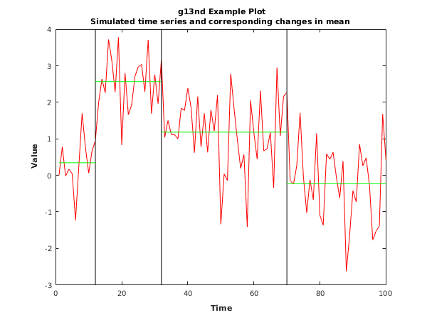
This example identifies changes in the mean, under the assumption that the data is normally distributed, for a simulated dataset with

100

observations. A BIC penalty is used, that is

β = \log n \approx 4.6

, the minimum segment size is set to

2

and the variance is fixed at

1

across the whole input series.

Open in the MATLAB editor: g13nd_example

function g13nd_example


fprintf('g13nd example results\n\n');

% Input series
y = [ 0.00; 0.78;-0.02; 0.17; 0.04;-1.23; 0.24; 1.70; 0.77; 0.06;
      0.67; 0.94; 1.99; 2.64; 2.26; 3.72; 3.14; 2.28; 3.78; 0.83;
      2.80; 1.66; 1.93; 2.71; 2.97; 3.04; 2.29; 3.71; 1.69; 2.76;
      1.96; 3.17; 1.04; 1.50; 1.12; 1.11; 1.00; 1.84; 1.78; 2.39;
      1.85; 0.62; 2.16; 0.78; 1.70; 0.63; 1.79; 1.21; 2.20;-1.34;
      0.04;-0.14; 2.78; 1.83; 0.98; 0.19; 0.57;-1.41; 2.05; 1.17;
      0.44; 2.32; 0.67; 0.73; 1.17;-0.34; 2.95; 1.08; 2.16; 2.27;
     -0.14;-0.24; 0.27; 1.71;-0.04;-1.03;-0.12;-0.67; 1.15;-1.10;
     -1.37; 0.59; 0.44; 0.63;-0.06;-0.62; 0.39;-2.63;-1.63;-0.42;
     -0.73; 0.85; 0.26; 0.48;-0.26;-1.77;-1.53;-1.39; 1.68; 0.43];

% Type of change point(s) being looked for
% (change in mean, assuming a Normal distribution)
ctype = int64(1);

% Standard deviation to use for Normal distribution
param = 1;

% The routines used in this example issue warnings, but return
% sensible restults, so save current warning state and turn warnings on
warn_state = nag_issue_warnings();
nag_issue_warnings(true);

[tau,sparam,ifail] = g13nd( ...
                            ctype, y, 'param', param);

% Reset the warning state to its initial value
nag_issue_warnings(warn_state);

% Print the results
fprintf('  -- Change Points --         --- Distribution ---\n');
fprintf('  Number     Position              Parameters\n');
fprintf(' ==================================================\n');
for i = 1:numel(tau)
  fprintf('%5d%13d%16.2f%16.2f\n', i, tau(i), sparam(1:2,i));
end

% Plot the results
fig1 = figure;

% Plot the original series
plot(y,'Color','red');

% Mark the change points, drop the last one as it is always
% at the end of the series
xpos = transpose(double(tau(1:end-1))*ones(1,2));
ypos = diag(ylim)*ones(2,numel(tau)-1);
line(xpos,ypos,'Color','black');

% Plot the estimated mean in each segment
xpos = transpose(cat(2,cat(1,1,tau(1:end-1)),tau));
ypos = ones(2,1)*sparam(1,:);
line(xpos,ypos,'Color','green');

% Add labels and titles
title({'{\bf g13nd Example Plot}',
       'Simulated time series and corresponding changes in mean'});
xlabel('{\bf Time}');
ylabel('{\bf Value}');

g13nd example results

  -- Change Points --         --- Distribution ---
  Number     Position              Parameters
 ==================================================
    1           12            0.34            1.00
    2           32            2.57            1.00
    3           70            1.18            1.00
    4          100           -0.23            1.00

This example plot shows the original data series, the estimated change points and the estimated mean in each of the identified segments.

PDF version (NAG web site, 64-bit version, 64-bit version)

Chapter Contents

Chapter Introduction

NAG Toolbox